Vector algebra in the analysis of genome wide expression data

comment

reviews

reports

deposited research

interactions

information

refereed research

Research

Vector algebra in the analysis of genome-wide expression data

Finny G Kuruvilla*, Peter J Park

†

_{and Stuart L Schreiber*}

Addresses: *Howard Hughes Medical Institute, Bauer Center for Genomics Research, Department of Chemistry and Chemical Biology,

Harvard University, Cambridge, MA 02138, USA. †_{Department of Biostatistics, Harvard School of Public Health, Informatics Program,}

Children’s Hospital, Harvard Medical School, Boston, MA 02115, USA.

Correspondence: Stuart L Schreiber. E-mail: [email protected]

Abstract

Background: Data from thousands of transcription-profiling experiments in organisms ranging from yeast to humans are now publicly available. How best to analyze these data remains an important challenge. A variety of tools have been used for this purpose, including hierarchical clustering, self-organizing maps and principal components analysis. In particular, concepts from vector algebra have proven useful in the study of genome-wide expression data.

Results: Here we present a framework based on vector algebra for the analysis of transcription profiles that is geometrically intuitive and computationally efficient. Concepts in vector algebra such as angles, magnitudes, subspaces, singular value decomposition, bases and projections have natural and powerful interpretations in the analysis of microarray data. Angles in particular offer a rigorous method of defining ‘similarity’ and are useful in evaluating the claims of a microarray-based study. We present a sample analysis of cells treated with rapamycin, an immunosuppressant whose effects have been extensively studied with microarrays. In addition, the algebraic concept of a basis for a space affords the opportunity to simplify data analysis and uncover a limited number of expression vectors to span the transcriptional range of cell behavior.

Conclusions: This framework represents a compact, powerful and scalable construction for analysis and computation. As the amount of microarray data in the public domain grows, these vector-based methods are relevant in determining statistical significance. These approaches are also well suited to extract biologically meaningful information in the analysis of signaling networks. Published: 13 February 2002

GenomeBiology2002, 3(3):research0011.1–0011.11

The electronic version of this article is the complete one and can be found online at http://genomebiology.com/2002/3/3/research/0011 © 2002 Kuruvilla et al., licensee BioMed Central Ltd

(Print ISSN 1465-6906; Online ISSN 1465-6914)

Received: 20 August 2001 Revised: 14 December 2001 Accepted: 11 January 2002

Background

The three goals of most microarray experiments are descrip-tion, classificadescrip-tion, or characterization. For example, microarrays have been used to describe comprehensively the diauxic shift, progression through the cell cycle, sporulation and the effects of treatment with a small molecule [1-4]. They have been used to classify the cancer type of a given sample or classify groups of co-regulated genes [5-8]. Finally, microarrays have been used to characterize biologi-cal systems using comparisons of wild-type and mutant cells, with the goal of obtaining mechanistic insights [9-11].

As the number of publicly available profiles in Saccha-romyces cerevisiae alone now exceeds 500, a great need exists to exploit this information properly to understand cell function. At least three independent international projects have been set up to serve as database-driven repositories of genome-wide expression data [14]. A major effort is being made to systematize data storage, especially involving XML (extensible markup language), to ensure interoperability of these databases and associated analysis tools.

A related need that has been less addressed is the systemati-zation of expression data analysis. This requirement extends not only to analysis but also to pedagogy and to practical aspects of algorithm implementation. Various studies in the literature have successfully implemented tools from vector algebra in analyzing genome-wide expression data [11,15,16]. However, a framework for the analysis of transcription pro-files using vector algebra has not yet been codified. Here we present such a framework. Common statistical measures have natural counterparts in vector algebra that have visual interpretations and are easily implemented on a computer. Within this framework, the analysis of genome-wide expres-sion data is converted to the study of high-dimenexpres-sional vector spaces. The many powerful theorems that have been developed in vector algebra can be applied to these spaces, and these theorems offer biologically relevant insights. Ele-ments of the vector space can also be analyzed statistically. This construction has analytic and pedagogic appeal.

Results and discussion

Transcription-profiling experiments offer different kinds of measurements depending on the technology used. One type of technology (using noncompetitive hybridization) mea-sures absolute gene expression, while a second type (using competitive hybridization) measures relative gene expres-sion. A microarray that uses competitive hybridization yields a list of fold changes for each gene between the conditions or cell types measured. The data from a microarray that uses noncompetitive hybridization can be ‘divided’ (after proper normalization) into another microarray of the same type to produce the fold change of each gene from one condition to another. In practice, even those investigators who use non-competitive technology platforms generally interpret and publish the fold changes between conditions or strains rather than absolute gene-expression levels. Therefore this study will focus on analysis of fold-change values, hereafter called a transcription or expression profile.

There are three common types of values that can be associ-ated with the fold change of a gene. The first, a signed fold change (such as a +1.6 or -2.3 fold change, corresponding to induction or repression, respectively) has the most intuitive appeal but has a discontinuity spanning from -1.0 to +1.0 that can be problematic. The second type, an unsigned fold

change (such as 1.6 or 0.43 fold change, again correspond-ing to induction or repression, respectively) has no such discontinuity but is bounded on the left by zero and is unbounded on the right. This asymmetry about unity hinders analysis. The third type, a logarithm (base 2, base 10, or natural) of the unsigned fold change, is undoubtedly the most tractable. No fold change in expression is repre-sented by zero, induction is positive and repression is nega-tive. Most importantly, there are no discontinuities or asymmetries.

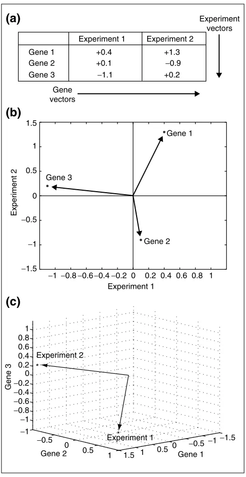
Once a set of transcription profiles is obtained (where each profile represents a set of fold changes for a set of genes), a data matrix can be generated with genes as rows and experi-ments as columns (Figure 1a). With this picture in mind, generating vectors from the data matrix (the logarithms of the unsigned fold changes) is a natural operation for which there is an obvious construction.

Definition. For p transcription profiles measuring the expression of ngenes, let sijrepresent the logarithm of the

expression of the ith gene in the jth experiment. The vector

[si1si2…sip]T

is defined as a ‘gene vector’. Similarly,

is defined as an ‘experiment vector’. By construction, a gene vector is p-dimensional and an experiment vector is n-dimensional. An ‘expression vector’ represents either a gene vector or an experiment vector. The superscript T

desig-nates transposition.

It can easily be seen that with respect to the data matrix, a gene vector consists of the elements of a row and an experi-ment vector consists of the eleexperi-ments of a column (Figure 1a). By convention, vectors are treated as columns and not as rows. Experiment vectors are already columns, so gene vectors are transposed from rows to also become columns.

In the most common scheme of comparing two profiles, a ‘cloud’ of genes is plotted on a scatterplot. This view is simply the display of n two-dimensional gene vectors (Figure 1b). It is well suited to detecting particular genes whose expression varies between experiments. As more experiments are added to the matrix, the dimension of the space grows but the number of points remains fixed. Considering a large number of experiments, genes that have similar biological regulation remain in nearby regions of high-dimensional

s1j

s2j

comment

reviews

reports

deposited research

interactions

information

refereed research

spaces. Integrated with promoter-sequence analysis and con-sideration of chromatin structure, the study of gene vectors is useful in studies of transcription regulation.

There is another, complementary, way of thinking about expression profiles, or more generally, about multivariate statistical data [17]. Although analysis of gene vectors is a powerful tool, it is less efficient at demonstrating relation-ships between profiles. This is because overlaying clouds of thousands of gene vectors may not offer an insightful picture because of the many data points in view. In the alternative method of analysis, an expression profile is regarded as just one point in a high-dimensional space. Because this point captures the same information con-tained in the scatterplot of gene vectors, the point must reside in a much higher-dimensional space. In this space, the relationships between profiles become more apparent. Instead of plotting genes, one now plots experiments (Figure 1c). As new profiles are added to the data matrix, the dimension of the space remains fixed but the number of points increases, the reverse case of gene vectors. Although the high-dimensional space of experiment vectors cannot be visualized, the relationships of vectors in the space can often be understood using intuition from the two- or three-dimensional case. The power of vector algebra comes from its ability to scale - the concepts, equa-tions and theorems move seamlessly (usually identically) to higher dimensions.

Assuming that there are ngenes represented on the microar-ray, it is theoretically possible that each profile would yield an n-dimensional experiment vector. However, because of poor detection of scarce transcripts, flaws on the microarray or experimental error, an expression profile in practice gives fewer than nvalues. This leaves three basic options for how to carry out the analysis. The first is that a lack of data can be declared as no change in expression, and a zero inserted into the position of that gene. This approach is generally too simplistic for use in further analysis.

The second option is to estimate the missing value on the basis of other profiles and insert it into the vector. For example, we can look for the gene most similar to the missing gene as judged by all other experiments, and then replace the missing value with the value of the similar gene for that experiment. For robustness, we can also find the most similar kgenes and use the average of those genes for that experiment as the replacement. A comparative study has found that this k-nearest neighbors method performs better than filling missing values with zeros or the averages of that gene in other experiments [18]. There are more complicated imputation methods in the statistics literature, but their usefulness, given the complex calculations involved, is not yet clear.

Finally, the vector space can be resized to a smaller dimen-sion than n, where the expression profiles of interest have data for all genes in that space. As the missing data are not estimated, this is the most conservative method of analysis, although at the price of discarding some data.

Figure 1

The two complementary methods of understanding a transcription profile. (a)Two transcription profiles of three genes are shown. Rows form gene vectors while columns form experiment vectors. (b)In a typical profile comparison, gene vectors are plotted in two dimensions, where the axes represent the experiments and the points are the genes. Data from (a) are plotted. Additional genes add points to the graph, but it remains in two dimensions. (c)In the vector-based approach, the axes are genes and the points are experiments. Data from (a) are also plotted here. Additional genes would not add any points to the graph (that is, there would always only be two vectors), but the space that the vectors reside in would increase in dimension.

Gene 1

Experiment 1

−1.1 +0.2

+0.1 −0.9

+0.4 +1.3

Gene 2 Gene 3

Experiment 2

−1−0.8−0.6−0.4−0.2 0 0.2 0.4 0.6 0.8 1

Gene 1

Gene 2 Gene 3

Experiment 1

Experiment 2

−1.5

−1

−0.5 0 0.5 1 1.5

−0.5 0

0.5 1 0

Experiment 1 Experiment 2

Gene 1 Gene 2

Gene 3

Experiment vectors

Gene vectors

*

*

−1.5

−1

−0.5 0 0.5 1 1.5

−1

−1

−0.8

−0.6

−0.4

−0.2 0.2 0.4 0.6 0.8 1

(a)

(b)

Vector angle is the counterpart to the Pearson correlation coefficient

One of the most fundamental measures in statistics is the Pearson correlation coefficient (referred to as r). This repre-sents a widely used measure of similarity between n-tuples. With expression vectors, the geometric picture of similarity is that the vectors are pointing in the same direction of expression space. This picture is equivalent to two vectors with a small angle between them. When expression vectors are uncorrelated, they are orthogonal. This leads to the fol-lowing remark.

Remark 1. Correlation of expression vectors corresponds to the angle q between those vectors. Low angle (r near 1) implies correlation, Angle near 90° (r near zero) implies uncorrelation, and angle near 180°(rnear –1) implies anti-correlation.

This remark is motivated by consideration of the relation-ship between the Pearson correlation coefficient (r) and vector angle (q). (We use the notation where < , > represents an inner product, also called a dot product, and where cov( , ) is the covariance between ordered n-tuples.) For two vectors Nand O, the formulas for rand qare:

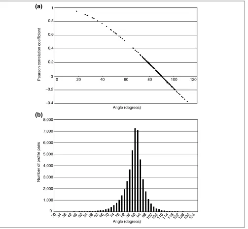
It is evident that r and the argument of the inverse cosine function are identical except that covariance and inner product are interchanged. In practice, the argument to the inverse cosine and rare nearly identical because the covari-ance is essentially a mean adjusted inner product and the means of expression vectors are near zero. (In fact, covari-ance and inner product are identical for vectors with zero mean.) Thus, there is no advantage of either measure because of nearly identical performance on actual expression data (Figure 2a).

For gene vectors, angles are a measure of how similar two genes are expressed across experiments. For experiment vectors, angles are a measure of how similar two experi-ments are across genes. For experiment vectors, a quantita-tive sense of the distribution of q can be obtained by examining a collection of diverse transcription profiles. A set of 300 transcription profiles in S. cerevisiae from a wide variety of gene deletions and treatments was obtained and made publicly available [19]. We converted these profiles into experiment vectors and computed all possible angles between the vectors (a total of 44,850 angles). (Computer source written in Matlabä is publicly available at our website [20]) These angles gave a distribution with a mean of 88.4° (close to orthogonal, as expected) and a standard deviation of 7.4°(Figure 2b). In practice, we have found 60°

and 120° as useful cutoff values for significance of correla-tion or anticorrelacorrela-tion, respectively.

The vector algebra approach is illustrated using a publicly available data set. The small molecule rapamycin has been transcriptionally profiled by three research groups in four separate studies [4,11,21,22]. It has a very dramatic expres-sion profile in which hundreds of genes are rapidly (within minutes) up- or down-regulated. The protein targets of rapamycin (the Tor proteins) are known to sense nutrients. When treated as an experiment vector, other experiment vectors were searched for that had a low angle with the rapamycin vector. Against the same set of 300 diverse expression profiles described earlier [19], not a single vector could be found that had an angle less than 60° with the rapamycin experiment vector (data not shown). However another study identified two vectors with smaller angles to the rapamycin expression vector (angles of 44°and 47°) [11]. These similar vectors were those corresponding to the removal of high-quality carbon or nitrogen from the media. Thus, it can be inferred that the Tor proteins regulate the responses to carbon- and nitrogen-quality of the medium. This is an example of using angles to identify the functions of uncharacterized proteins.

It is apparent that angles provide a quantitative measure for asserting genome-wide similarities. This measure is impor-tant when making claims about the target of a small mole-cule, effects of gene deletion or specificity of a drug. Orthogonal angles (implying uncorrelation) when similarity is expected or claimed raise questions about the validity of the hypothesis under examination.

A ratio of magnitudes is a natural second metric for comparing two expression vectors

An advantage of vector algebra is the extension from angles into ratios of magnitudes for which other formulations have awkward or no counterparts. The two four-dimensional vectors N= [1 0 2 -1]T_{and O= [2 0 4 -2]}T_{have q= 0}

(imply-ing r = 1). However, there is an important difference between the vectors not identified by these measures, as we can observe that O = 2N. This information is captured by computing the ratio of vector magnitudes.

Remark 2. Besides angle, the ratio of vector magnitudes (a) is a second measure of similarity of two expression vectors. For two vectors Nand O, this is calculated as:

With the two four-dimensional vectors listed above, ais easily seen to be 2. By interchanging < , > and cov( , ) as was done with r and q, it is tempting to think that the quantity b= (cov(O,O)/cov(N,N))1/2_{might behave similarly}

<O,O> a= ———— <N,N> cov(N,O) <N,O>

r= ———————————— q= cos–1 _{——————————}

to a. With the same vectors as above, b = a = 2. When considering the two vectors N= [2 2 2 2]T_{and O= [1 2 1 2]}T_,

it can be calculated that a= 0.79, the value expected as Ois a ‘smaller’ vector. However b = 0.5/0 = ¥. Indeed, the mean subtraction component of the covariance fundamen-tally alters the behavior of b compared to a, making it an unsuitable measure of expression vector magnitude. An elegant feature of regarding microarray data as expression

vectors is that both angles and magnitudes are natural measurements with important biological meaning, as will be discussed in later sections.

Searching subspaces is an important step in analyzing expression vectors

Another advantage to treating expression data as vectors in a space rather than as n-tuples is the associated notion of

comment

reviews

reports

deposited research

interactions

information

refereed research

Figure 2

The relationship between the Pearson correlation coefficient and angle, and the statistical distribution of angles. (a)The Pearson correlation coefficients and the angles between 180 pairs of actual transcription profiles were computed. Plotting one measure against the other reveals their close relationship. (b)The statistical distribution of angles in a large, diverse data set (300 profiles) [19] was computed by calculating angles between all possible pairs (a total of 44,850 angles) of expression vectors. Data were taken from the Rosetta Inpharmatics website [34] and the software used to compute the angles is publicly available for download from our website [20].

−0.4 −0.2 0 0.2 0.4 0.6 0.8 1

0 20 40 60 80 100 120

Angle (degrees)

Angle (degrees)

Pearson correlation coefficient

0 1,000 2,000 3,000 4,000 5,000 6,000 7,000 8,000

30 34 38 42 46 50 54 58 62 66 70 74 78 82 86 90 94 98 102 106 110 114 118 122 126 130 134

Number of profile pairs

(a)

subspaces. With experiment vectors, this concept is particu-larly valuable. Experiment vector space can be divided into subspaces, most naturally where the subspaces correspond to co-regulated or functionally related genes. This can most easily be done using annotated lists where genes are classi-fied by function. The Munich Information Center for Protein Sequences (MIPS) provides a commonly used functional grouping for genes [23].

Considering subspaces is nearly always an essential part of analysis. From the vantage point of certain subspaces, many different experiment vectors may ‘collapse’ into identical vectors. This enables the decomposition of vectors into sums of common and distinct components. For example, yeast stress responses (such as DNA damage or heat shock) are composed of a general response that stresses share and a specific response for the particular stress faced. Identification of these subspaces remains a goal in biology. Another example is that of the Tor proteins, which have many effectors, one of

which is called Ure2p. Comparing the expression vectors of rapamycin treatment with a URE2deletion reveals that the genome-wide angle between these two vectors is 76° and thus the vectors show only weak correlation. However, cal-culating the angle of these same vectors within the subspace of genes controlled by Ure2p gives an angle of 13°[11]. With respect to this subspace of genes, treatment with rapamycin and deletion of URE2 are nearly identical. Experiments reveal that treatment with rapamycin leads to dephosphory-lation of Ure2p, corroborating this low angle [4,21]. Thus it is important to consider not only whole-genome angles, but also those for important subspaces.

The effects of mutations on vector angles and magnitudes

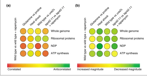
When studying a particular process by transcription profil-ing, it is common also to transcriptionally profile the same process after deleting one or more genes known to be involved. For example, this has been carried out with MAP Figure 3

An illustration of the use of the colorimetric comparison array (CCA) to infer information about a cellular signaling network. (a)Using competitive hybridization data from a study of the target of rapamycin (Tor) proteins) [11], the angles between a reference expression vector of a wild-type strain treated with rapamycin and four other expression vectors are represented on a CCA. The profile of cells shifted from glutamine to proline shows that at a whole-genome level, and within the subspaces shown, there is strong similarity (44°at a whole-genome level) to a profile of cells treated with rapamycin. Cells that have undergone heat shock, however, have an orthogonal (uncorrelated) expression vector. Deleting the gene URE2(ure2D) does not generate whole-genome correlation, but does generate correlation within the subspace of nitrogen-discrimination pathway (NDP) genes. Finally, cells containing the tap42-11 allele of TAP42that are treated with rapamycin illustrate that Tap42p is downstream of the Tor proteins in the control of ribosomal protein gene expression. (b)A similar analysis to that in (a) can be carried out using ratios of vector magnitudes (a). The overall greenness of the CCA reflects the fact that these four expression vectors have a smaller magnitude than the reference rapamycin-treatment profile. The magnitude of the whole-genome expression vector of heat shock is considerably smaller. Deleting URE2, however, increases the magnitude of expression of the NDP subspace of genes to levels comparable to those of cells treated with rapamycin. When TAP42is mutated to the tap42-11allele, NDP gene induction is severely impaired, implicating Tap42p as an important regulator of NDP gene expression downstream of the Tor proteins. Iterating this analysis over many effectors and many subspaces of genes reveals a wealth of information about the transcriptional network downstream of the Tor proteins [11].

Glutamine vs prolineHeat shockWild type vs

ure2

∆

tap42-11

vs

tap42-11

+ rapamycin Glutamine vs prolineHeat shockWild type vs

ure2

∆

tap42-11

vs

tap42-11

+ rapamycin

Whole genome

Ribosomal proteins

NDP

ATP synthesis

Whole genome

Ribosomal proteins

NDP

ATP synthesis

Wild type vs wild type + rapamycin Wild type vs wild type + rapamycin

Correlated Anticorrelated Increased magnitude Decreased magnitude

kinase deletion mutants after pheromone treatment [10], deletions of effectors of the Tor proteins after rapamycin treatment [11], and lexAdeletions after UV irradiation [24].

When an effector of some process is deleted, the resulting vector is often not uncorrelated in the subspace involving that effector, but is reduced in magnitude. For example, when there are two transcription factors with overlapping specificity for some genes, deletion of one can be compen-sated by the presence of the second with a similar (though weaker) induction of the same genes. If an effector truly is an exclusive controller of some set of genes, when it is deleted, the resulting experiment vector in that subspace would be expected to be orthogonal (uncorrelated) with the original vector. However, biological networks generally exhibit redundancy in their control of genes - a reduction in the vector magnitude is to be more commonly expected than rotation toward perpendicularity (uncorrelation). Thus it is important to rely on the coordinate use of angles and magni-tudes in expression-profiling analysis, something that is not always performed in the literature.

Combined use of angles and ratios of vector magnitudes is a tool for biological discovery

When one is characterizing a transcription profile of an uncharacterized gene deletion or treatment with a small molecule, the first operation that should ordinarily be com-pleted is a comparison of that profile as an experiment vector with all other available experiment vectors from the same organism. By performing such a comparison, the gene can be partially characterized or the target of a small mole-cule can be identified [19]. By coloring the results of a com-parison, mimicking the false-coloring schemes usually found on microarrays, one can quickly scan a large set of profiles for those correlated, uncorrelated, or anticorrelated with a reference profile that is being tested [11]. This color scheme is red to represent correlation, yellow to represent uncorre-lation, and green to represent anticorrelation (Figure 3). This overall depiction is called a colorimetric comparison array (CCA). It can also be carried out with ratios of vector magnitudes where red represents greater magnitude, yellow unchanged magnitude, and green reduced magnitude.

To understand the most general relationships, it is useful in the first row of a CCA to compare whole-experiment vectors. This gives an important genome-wide characterization of the profiles being studied - assertions of global behavior should be substantiated in these values. As previously discussed, the angles and magnitudes within subspaces are important to analyze - in subsequent rows, therefore, the same experiment vectors are compared in various subspaces of the genome. By examining a range of subspaces, this analysis can be used to partition a transcription profile and define which effectors are responsible for particular patterns of expression. By looking at whole-genome angles as well as angles within subspaces of interest, the CCA reveals a wealth of information about the

expression vectors being studied (Figure 3). A CCA can also be used to identify the structure of signaling networks.

Singular value decomposition in expression-profile analysis

We next explore ideas relating to dimensionality reduction of expression vectors. Dimensionality reduction is a common problem in many disciplines of science and engi-neering. Questions include: what are the essential pieces of information within a transcription profile and what is noise? If the full set of genes (around 6,000 in S. cerevisiae) carries redundant information, how small a subset can we choose? Are most transcription profiles merely combinations of a smaller number of transcription profiles? The first tool we discuss is singular value decomposition (SVD).

SVD is a matrix factorization that reveals many important properties of a matrix. It is a standard tool in many areas of the physical sciences, and many algorithms in matrix algebra make use of SVD. Given an n´prectangular data matrix )n´p of expression profiles (again where n is the

number of genes, pis the number of experiments), we can obtain the following factorization:

T

)n´p= 7n´n,n´p8p´p

where 7and 8are orthonormal and ,is diagonal. (Mathe-matical details of the SVD can be found in Materials and methods.) The intuition behind the SVD is straightforward. Let Kibe the ith column of 7. Note that this column vector is

n-dimensional. The best vector (in a sense that can be made mathematically precise, see Materials and methods) that captures (spans) the experiment vectors of )is K1. Similarly,

the best two column vectors that span the experiment vectors of ) are K1 and K2. In the limit, all n vectors Ki

exactly span all the experiment vectors of ). In the same way, the columns of 8, in descending order, are p-dimen-sional vectors that best span the gene vectors of ). These ideas are best illustrated with an example.

The first column of 7, K1, best spans (that is, when

multi-plied by a constant) the columns of ). Together with the second column, )is exactly captured by taking linear com-binations of K1 and K2. In this case, K3 and K4 are not

comment

reviews

reports

deposited research

interactions

information

refereed research

2 4 1 3 0 0 0 0

0.82 –0.58 0 0 0.58 0.82 0 0

0 0 1 0

0 0 0 1

5.47 0 0 0.37

0 0

0 0

needed to capture ). Similarly, the first column of 8, L1,

best spans the gene vectors (rows) of ). The first value along the diagonal of ,measures how much contribution K1 and L1make to capturing ), and the next value

mea-sures how much contribution K2and L2make. In this case,

the large size of the first singular value indicates that K1

and L1capture most of the information in ). These values

along the diagonal of ,are called the singular values of ). Matrices that contain mostly redundant columns (low-rank matrices) have singular values that rapidly decay, because the matrix is efficiently spanned by a small number of vectors. However, matrices containing very independent columns (high-rank matrices) have singular values that slowly decay. In the limit, the identity matrix, which has the highest possible rank of n, has singular values that do not decay at all - they all are one.

For microarray data, SVD can be used to bring out domi-nant underlying behaviors. For example, examining the cell-cycle data [25] using SVD revealed that among the first 7 vectors (K1, K2, …), the first corresponds to a

steady-state and the subsequent ones correspond to the oscillatory behavior that one would expect from such data [15,16]. SVD can also be used to ‘de-noise’ profiles by recomputing the data matrix using only significant Kivectors

(signifi-cance determined by reading the ith singular value along the diagonal matrix ,.) The SVD can also be used to esti-mate missing values.

A technique called principal components analysis (PCA) [26] is closely related to the SVD. In PCA, the factorization is applied to the covariance matrix of the data rather than the original data matrix. If the data are mean-adjusted, both SVD and PCA give the same information. If the data are from a time series, then the principal components may corre-spond to derivatives of the data [27].

Towards a basis of expression vectors

One of the most powerful ideas in linear algebra is the notion of basis vectors. Besides constructing the space, basis vectors can be chosen to highlight important features of the data or simply to store the data efficiently. For example, the function sin xcan be expressed either in a polynomial or exponential basis,

x3 _x5 _x7

sin x= x– —— + —— — —— + …

3! 5! 7!

1

sin x= —

冢

冣

2

The first basis is clearly awkward - it is infinite-dimensional and offers little insight. However, the second basis captures the sine wave more compactly and provides more insight. Many of the successes of vector algebra in image compres-sion, smoothing and signal detection come from the identifi-cation of appropriate basis functions.

This concept has important implications in the analysis of transcription-profiling data. Considering the data as expres-sion vectors, what is the right basis to express the data in? The data is originally in the basis of genes. But is that the best basis? We have already examined one change of basis -the SVD. In this case, -the Kiand Livectors are basis vectors

for the spaces of experiment vectors and gene vectors, respectively. While very efficient basis vectors, the vectors themselves are completely artificial and do not correspond to actual profiles.

An important question in biology is how many different fun-damental cellular states or transitions exist. It may be that there are a relatively small number, and that cellular states or transitions are essentially superpositions of a finite number of basic states or transitions. This question is easily posed in expression space because, if the hypothesis holds, the complete set of expression profiles can be examined for the smallest number of basis vectors that can construct the nearly identical entire set. If a profile is added to the data matrix and cannot adequately be constructed by other exist-ing profiles, then it becomes a basis vector. The collection of basis vectors formed by this procedure can be thought of as containing the building blocks of cellular state or transition space. Thus, it would be interesting to try to find basis vectors for all experiment vectors, using actual experiment vectors and not artificial bases that offer little insight.

First, how can one estimate how many basis vectors are required? This problem corresponds to estimating the rank of the data matrix. This problem of finding an approximate rank of a matrix, k, is a common one. SVD, as described above, is often employed. Using SVD, one typically looks for a sharp drop in the singular values to estimate the rank. Let us suppose that the singular values fall below a defined threshold at some value. This value serves as a logical choice for k. In fact, the first kvectors Kiof )serve as the best

pos-sible basis to span ). In our case, however, we desire the basis vectors to be a subset of the original vectors of ). This is a more difficult problem.

We investigated these concepts using two large data sets of transcription profiles generated in S. cerevisiae: the set of 300 expression profiles previously analyzed and a second set of over 170 expression profiles of various yeast environ-mental responses [19,28]. We converted these sets to data matrices of experiment vectors and computed the singular values of each matrix. For each matrix, the singular values decayed rapidly (Figure 4). This decay shows that the columns of the matrix are far from orthogonal and a basis containing a small number of Ki vectors can efficiently

further suggests that there are a small number of building-block transitions that yeast can undergo and that other behaviors are, at least partially, superpositions of these transitions.

But how can one find these building-block, fundamental expression vectors in the profile set? Instead of using the Ki

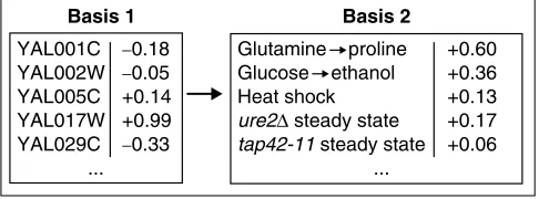
vectors from SVD (which are linear combinations of the experiment vectors) it would be useful to identify which actual experiment vectors are most useful to form a basis for the matrix. That is, it would be useful to express pro-files in terms of other propro-files (basis vectors), rather than simply as lists of genes (Figure 5). There are a number of possible algorithms for identifying these basis experiment vectors. We tested a variety of algorithms, especially those

utilizing projections of the Ki vectors on ), to identify

optimal candidate basis vectors. (The source code for one such algorithm is publicly available online at [20].) While small subsets of experiment vectors could span the entire set of experiment vectors, it was found that there were many such subsets of experimental vectors that had a com-parable spanning ability toward )(data not shown). This suggests that the cell probably does have a small number of fundamental transitions, although many different groups of transitions (as represented by experiment vectors) appear nearly equivalently able to span the transcriptional range of cellular behavior.

Given this behavior, perhaps the ideal basis vectors for tran-sition space would be the basis of experiment vectors in which only one signaling pathway is selectively modulated. This could be accomplished with small molecules like rapamycin that selectively modulate one signaling pathway with complete specificity. If one had a collection of small molecules that could selectively modulate every signaling pathway in the cell, then it might be possible to simply project an experiment vector on these small molecules’ experiment vectors and determine which pathways are acti-vated and to what degree. This would immediately charac-terize the expression profile in a very powerful basis that provides a great deal of biological insight.

Conclusions

We have described various techniques motivated by vector algebra for analyzing genome-wide expression data. Some of these techniques have been used previously, but we find that

comment

reviews

reports

deposited research

interactions

information

refereed research

Figure 4

Using the SVD to estimate the number of fundamental expression vectors required to efficiently span a profile set. (a)A set of 300 diverse expression profiles [19] was converted to a matrix of expression vectors and the singular values were computed, normalizing such that the first singular value was equal to 1. (b)A set of 173 profiles of various yeast environmental responses [28] were converted to a matrix of expression vectors and processed as in (a).

0 50 100 150 200 250 300 0 20 40 60 80 100 120 140 160

Singular value number Singular value number

Singular value

0 0.1 0.2 0.3 0.4 0.5 0.6 0.7 0.8 0.9 1

Singular value

0 0.1 0.2 0.3 0.4 0.5 0.6 0.7 0.8 0.9 1

(a)

(b)

Figure 5

The transcriptional profile of rapamycin expressed in two alternate bases. A part of the traditional basis for a transcription profile is shown on the left (only five genes out of around 6,000 are shown). The experiment vector of treatment with rapamycin was projected onto the five experiment vectors shown on the right. The coefficients for the rapamycin expression vector in this five-dimensional basis are shown on the extreme right.

YAL001C −0.18 YAL002W −0.05 YAL005C +0.14 YAL017W +0.99 YAL029C −0.33 ...

Glutamine proline +0.60 Glucose ethanol +0.36

Heat shock +0.13

ure2∆ steady state +0.17 tap42-11 steady state +0.06 ...

by regarding expression profiles as vectors, either in the sense of genes or experiments, we gain a richer understand-ing of the existunderstand-ing techniques and can take these insights into new directions.

The angle between two vectors is essentially equivalent to the Pearson correlation coefficient and studying the changes in magnitudes as well as the angles provides important bio-logical information. In particular, we find that decomposing the experiment vector space into a set of smaller subspaces, using functional categories for instance, results in a concise but useful description of the biological system (Figure 3). These types of genome-wide descriptions are essential for understanding large amounts of complex expression data. Thinking in terms of vector spaces naturally introduced the idea of optimal basis vectors, but with the constraint that these basis vectors belong to the original set of expression vectors. This may be a useful way of characterizing expres-sion profiles. We have described the usefulness of the singu-lar value decomposition as a tool for reducing the dimension of the problem and the insight it brings to the problem of finding basis vectors.

A complete analysis of genome-wide expression data involves numerous issues not discussed here. The impor-tance of preprocessing and normalization to correct for various artifacts has been noted recently [29,30]. Artifi-cially large fold changes caused by small values in ratios (red/green or vice versa) should be numerically bounded in competitive hybridization experiments. Assigning a level of significance to observed changes in expression levels is also an important issue and has been addressed by a number of different approaches, most often with a deriva-tion of a statistical model for noise to obtain estimates for the fold changes [31,32]. For oligonucleotide arrays, there are similar and sometimes more complicated issues for the same steps. Finally, there are a variety of clustering and data-mining techniques for understanding the structure of the data in other ways. Appropriate methods should be chosen carefully, depending on the type of data and the questions to be answered. As the quantity of expression data increases rapidly, more tools such as the ones devel-oped here will play an important role in understanding biological states and transitions.

Materials and methods

Computer software was written in the Matlab™ program-ming language and is publicly available for download from our website [20].

Singular value decomposition (SVD) SVD is the matrix factorization:

T

)n´p= 7n´n,n´p8p´p

where ,is diagonal and 7and 8are orthonormal (77T₌

7T_{7= 1}

n´nand 88T= 8T8= 1p´p). The diagonal entries of ,

are the singular values s1³s2³… ³spand the columns {Ki}i

=1,…,nof 7and {Li}i=1,…,pof 8are called left and right

singu-lar vectors, respectively. For microarray data, we assume that n> pas we usually think of the data matrix as having n rows for genes and prows for experiments, and we assume that the columns are linearly independent.

The geometric visualization of the SVD is the following. When )n´pis applied to a p-dimensional sphere, the result is

an n-dimensional ellipse in which the principal axes have been stretched by factors s1,…, sp in directions K1,…,Kp

respectively. (The right singular vectors Liare the axes of the

sphere that get mapped to Kithrough )Li= siKi.) The

useful-ness of the SVD is often based on the fact that it answers the following important question: what is the best approxima-tion to )using a matrix of lower rank? (The term ‘best’ can be defined mathematically.) This is important because a comparable matrix with a smaller rank may make the under-lying structure of the matrix more apparent. Another way of writing )=7,8T_is:

p

T

)=

兺

Then, it can be shown mathematically that the best approxi-mation of dimension kis obtained by the partial sum of the first kterms [33]. Sometimes the terms siKiLiTare called the

‘characteristic modes’. This representation is similar to that of a signal by a sum of its Fourier modes. The SVD can be used to de-noise the data by recomputing the sum with the small singular values set to zero.

Measuring basis quality

Let )be an n´pmatrix where the columns of )represent a collection of ptranscription profiles over ngenes. k expres-sion vectors are chosen from )as a basis for the complete set. Let *be the matrix whose columns consist of the k expres-sion vectors (*is therefore n´k). The ability of *to form a basis for the remaining p- kvectors of )(designated Ni) is

tested by application of the projection theorem. Let 2be the projection matrix for *, that is 2= *(*T_*)-1_*T_{. A measure of}

the spanning ability of the basis *toward the Niis:

p–k _冨(1–2)N i冨

g=

兺

i=1 冨N_i冨

Until g is below a determined threshold for the original matrix ), a different collection of kexpression vectors can be tested or kcan be increased to include more basis vectors.

In the expression for g, the numerator is the ‘residual vector’, the part of the Nithat could not be captured by *. The

References

1. DeRisi JL, Iyer VR, Brown PO: Exploring the metabolic and genetic control of gene expression on a genomic scale. Science 1997, 278:680-686.

2. Cho RJ, Campbell MJ, Winzeler EA, Steinmetz L, Conway A, Wodicka L, Wolfsberg TG, Gabrielian AE, Landsman D, Lockhart DJ, Davis RW: A genome-wide transcriptional analysis of the mitotic cell cycle.Mol Cell 1998, 2:65-73.

3. Chu S, DeRisi J, Eisen M, Mulholland J, Botstein D, Brown PO, Her-skowitz I: The transcriptional program of sporulation in budding yeast.Science 1998, 282:699-705.

4. Hardwick JS, Kuruvilla FG, Tong JK, Shamji AF, Schreiber SL: Rapamycin-modulated transcription defines the subset of nutrient-sensitive signaling pathways directly controlled by the Tor proteins.Proc Natl Acad Sci USA 1999, 96:14866-14870. 5. Golub TR, Slonim DK, Tamayo P, Huard C, Gaasenbeek M,

Mesirov JP, Coller H, Loh ML, Downing JR, Caligiuri MA, et al.: Molecular classification of cancer: class discovery and class prediction by gene expression monitoring. Science 1999, 286:531-537.

6. Ross DT, Scherf U, Eisen MB, Perou CM, Rees C, Spellman P, Iyer V, Jeffrey SS, Van de Rijn M, Waltham M, et al.: Systematic variation in gene expression patterns in human cancer cell lines.Nat Genet 2000, 24:227-235.

7. Perou CM, Sorlie T, Eisen MB, van de Rijn M, Jeffrey SS, Rees CA, Pollack JR, Ross DT, Johnsen H, Akslen LA, et al.: Molecular por-traits of human breast tumours.Nature 2000, 406:747-752. 8. Brazma A, Jonassen I, Vilo J, Ukkonen E: Predicting gene

regula-tory elements in silicoon a genomic scale.Genome Res 1998, 8:1202-1215.

9. Holstege FC, Jennings EG, Wyrick JJ, Lee TI, Hengartner CJ, Green MR, Golub TR, Lander ES, Young RA: Dissecting the regulatory circuitry of a eukaryotic genome.Cell 1998, 95:717-728. 10. Roberts CJ, Nelson B, Marton MJ, Stoughton R, Meyer MR, Bennett

HA, He YD, Dai H, Walker WL, Hughes TR, et al.: Signaling and circuitry of multiple MAPK pathways revealed by a matrix of global gene expression profiles.Science 2000, 287:873-880. 11. Shamji AF, Kuruvilla FG, Schreiber SL: Partitioning the

transcrip-tional program induced by rapamycin among the effectors of the Tor proteins.Curr Biol 2000, 10:1574-1581.

12. Clark EA, Golub TR, Lander ES, Hynes RO: Genomic analysis of metastasis reveals an essential role for RhoC. Nature 2000, 406:532-535.

13. Brazma A, Vilo J: Gene expression data analysis.FEBS Lett 2000, 480:17-24.

14. Brazma A, Robinson A, Cameron G, Ashburner M: One-stop shop for microarray data.Nature 2000, 403:699-700.

15. Holter NS, Mitra M, Maritan A, Cieplak M, Banavar JR, Fedoroff NV: Fundamental patterns underlying gene expression profiles: simplicity from complexity. Proc Natl Acad Sci USA 2000, 97:8409-8414.

16. Alter O, Brown PO, Botstein D: Singular value decomposition for genome-wide expression data processing and modeling. Proc Natl Acad Sci USA 2000, 97:10101-10106.

17. Wickens TD: The Geometry of Multivariate Statistics. Hillsdale, NJ: Lawrence Erlbaum Associates; 1995.

18. Troyanskaya O, Cantor M, Sherlock G, Brown P, Hastie T, Tibshirani R, Botstein D, Altman RB: Missing value estimation methods for DNA microarrays.Bioinformatics 2001, 17:520-525.

19. Hughes TR, Marton MJ, Jones AR, Roberts CJ, Stoughton R, Armour CD, Bennett HA, Coffey E, Dai H, He YD, et al.: Functional dis-covery via a compendium of expression profiles.Cell 2000, 102:109-126.

20. Stuart Schreiber laboratory [http://www.schreiber.chem.harvard.edu]

21. Cardenas ME, Cutler NS, Lorenz MC, Di Como CJ, Heitman J: The TOR signaling cascade regulates gene expression in response to nutrients.Genes Dev 1999, 13:3271-3279.

22. Bertram PG, Choi JH, Carvalho J, Ai W, Zeng C, Chan TF, Zheng XF: Tripartite regulation of Gln3p by TOR, Ure2p and phos-phatases.J Biol Chem 2000, 275:35727-35733.

23. Mewes HW, Heumann K, Kaps A, Mayer K, Pfeiffer F, Stocker S, Frishman D: MIPS: a database for genomes and protein sequences. Nucleic Acids Res 1999, 27:44-48. [http://www.mips.biochem.mpg.de/]

24. Courcelle J, Khodursky A, Peter B, Brown PO, Hanawalt PC: Com-parative gene expression profiles following UV exposure in

wild-type and SOS-deficient Escherichia coli. Genetics 2001, 158:41-64.

25. Spellman PT, Sherlock G, Zhang MQ, Iyer VR, Anders K, Eisen MB, Brown PO, Botstein D, Futcher B: Comprehensive identification of cell cycle-regulated genes of the yeast Saccharomyces cerevisiae by microarray hybridization. Mol Biol Cell 1998, 9:3273-3297.

26. Johnson RA, Wichern DW: Applied Multivariate Statistical Analysis. Upper Saddle River, NJ: Prentice Hall; 1998.

27. Raychaudhuri S, Stuart JM, Altman RB: Principal components analysis to summarize microarray experiments: application to sporulation time series.Pac Symp Biocomput 2000, 455-466. 28. Gasch AP, Spellman PT, Kao CM, Carmel-Harel O, Eisen MB, Storz

G, Botstein D, Brown PO: Genomic expression programs in the response of yeast cells to environmental changes.Mol Biol Cell 2000, 11:4241-4257.

29. Tseng GC, Oh MK, Rohlin L, Liao JC, Wong WH: Issues in cDNA microarray analysis: quality filtering, channel normalization, models of variations and assessment of gene effects.Nucleic Acids Res 2001, 29:2549-2557.

30. Yang YH, Dudoit S, Luu P, Speed TP: Normalization for cDNA microarray data. In Microarrays: Optical Technologies and Informatics. Edited by Bittner ML, Chen Y, Dorsel AN, Dougherty ER. Bellingham: International Society for Optical Engineering, 2001, 141-152.

31. Chen Y, Dougherty ER, Bittner ML: Ratio-based decisions and the quantitative analysis of cDNA microarray images. J Biomed Optics 1997, 2:364-374.

32. Newton MA, Kendziorski CM, Richmond CS, Blattner FR, Tsui KW: On differential variability of expression ratios: improving statistical inference about gene expression changes from microarray data.J Comput Biol 2001, 8:37-52.

33. Golub GH, van Loan CF: Matrix Computation. Baltimore, MD: Johns Hopkins University Press; 1996.

34. Rosetta Inpharmatics [http://www.rii.com]

comment

reviews

reports

deposited research

interactions

information