Thesis by
Jeffrey Paul Fingler
In Partial Fulfillment of the Requirements for the
degree of
Doctor of Philosophy
CALIFORNIA INSTITUTE OF TECHNOLOGY
Pasadena, California
2007
© 2007
Jeffrey Paul Fingler
ACKNOWLEDGEMENTS
I would like to my advisor, Professor Scott Fraser, for being the ideal mentor for me during my Ph.D. research. Through all the continual “threats” of a terminal Master’s degree, Scott has provided me with the freedom to explore in my research while still giving solid direction when I needed it. The most amazing thing is that Scott predicted where my research would be at the end of my thesis in one of the first meetings we ever had.
I would like to thank my committee members Professors Rob Phillips, Kerry Vahala, and Changhuei Yang for their continued patience and support since the time of my candidacy exam. Additional thanks go to Changhuei Yang for providing me with advice and lab space for more than two years in which I was missing lab space of my own.
The work in this thesis would not have been completed without the help of many people. I would like to thank Dr. Dan Schwartz, an ophthalmologist at UCSF, for acquiring funding for this project as well as providing guidance for the research progression. For the zebrafish experiments, Le Trinh was instrumental in teaching me to breed, handle, and mount these animals for imaging. Julien Vermot was very helpful in providing me with extra zebrafish for imaging when I did not have the time to breed some of my own. For the mice imaging, Carol Readhead was responsible for all of the details associated with the acquisition and handling of the animals, which allowed me to focus on only the imaging considerations and saving me a lot of time and effort. Special thanks also go out to Rusty Lansford, David Huss, and Greg Poynter for setting up some sample systems for me. Thanks also go out to my officemate, labmate, and fellow optical experimenter Jon Williams for all the experimental discussions over the years.
ABSTRACT
Diagnosis of ophthalmic diseases like age-related macular degeneration is very important for treatment of the disease as well as the development of future treatments. Optical coherence tomography (OCT) is an optical interference technique which can measure the three-dimensional structural information of the reflecting layers within a sample. In retinal imaging, OCT is used as the primary diagnostic tool for structural abnormalities such as retinal holes and detachments. The contrast within the images of this technique is based upon reflectivity changes from different regions of the retina.
This thesis demonstrates the developments of methods used to produce additional contrast to the structural OCT images based on the tiny fluctuations of motion experienced by the mobile scatterers within a sample. Motion contrast was observed for motions smaller than 50 nm in images of a variety of samples. Initial contrast method demonstrations used Brownian motion differences to separate regions of a mobile Intralipid solution from a static agarose gel, chosen in concentration to minimize reflectivity contrast.
TABLE OF CONTENTS
Acknowledgements ...iii
Abstract ...iv
Table of Contents... v
List of Figures ...vii
Chapter 1: Introduction... 1
1.1 Introducing Age-related Macular Degeneration... 1
1.2 Current Approaches to Disease Treatment... 11
1.3 Current Diagnostic Technologies and Limitations... 13
1.4 References ... 23
Chapter 2: Optical Coherence Tomography ... 25
2.1 Basics of Optical Coherence Tomography (OCT)... 25
2.2 Axial Resolution... 29
2.3 Acquiring Fringe Data to Create OCT Images... 33
2.4 SNR of Time Domain OCT ... 36
2.5 Spectral Domain OCT (SDOCT)... 38
2.6 SNR of SDOCT... 41
2.7 SDOCT Limitations ... 47
2.8 Phase Changes as Basis of Contrast ... 49
2.9 Choosing Between TDOCT and SDOCT... 51
2.10 References ... 53
Chapter 3: Tradeoffs and Experimental Methods... 55
3.1 OCT System Tradeoffs ... 55
3.2 Imaging Tradeoffs ... 65
3.3 Phase Contrast Tradeoffs ... 69
3.4 Phase Contrast Method: MB-scan ... 82
3.5 Phase Contrast Method: BM-scan ... 90
3.6 References ... 100
Chapter 4: Motion Contrast Imaging using Zebrafish... 101
4.1 Choosing Zebrafish as the Animal Model... 101
4.2 Creating SDOCT Images ... 103
4.3 Sample Preparation... 106
4.4 Bulk Motion Removal... 108
4.5 Zebrafish Tail Contrast Imaging: MB-scan versus BM-scan ... 110
4.6 Zebrafish Tail Motion Contrast over Time... 117
4.7 Segmental Vessel Imaging... 123
4.8 En face Images over Zebrafish Heart ... 126
Chapter 5: Mouse Retinal Imaging ... 131
5.1 Human Retinal OCT Imaging Explained ... 131
5.2 Differences between Human and Mouse Eye Imaging... 133
5.3 Aligning Retinal SDOCT Images ... 136
5.4 Phase Contrast Imaging... 138
5.5 En face Motion Contrast Images... 156
5.6 Improving BM-scan Capabilities... 164
5.7 Discussions of Human Contrast Imaging ... 171
5.8 References ... 174
LIST OF FIGURES
Figure Page
1.1. Side View Image of the Eye ... 2
1.2. Schematic Image of Retina ... 2
1.3. Daily Photoreceptor Renewal Process... 4
1.4. Lipid Content of Bruch’s Membrane versus Age ... 5
1.5. Electron Micrograph Images of Bruch’s Membrane... 6
1.6. Histology of Normal and Lipid-filled Retinas ... 6
1.7. Bruch’s Membrane Hydraulic Conductivity versus Age... 7
1.8. Bruch’s Membrane Permeability versus Age... 7
1.9. Fundus Photography Image of Healthy Eye... 8
1.10. Simulated Images of AMD Vision Loss ... 9
1.11. Wet AMD Schematic ... 10
1.12. AMD Prevalence Statistics for the United States... 11
1.13. Retinal Histology Comparison with Schematic Image ... 14
1.14. Snellen Chart for Visual Acuity Diagnostic... 15
1.15. Amsler Grid for Wet AMD Diagnostic ... 16
1.16. Fundus Photography Images for AMD Eyes ... 17
1.17. Fluorescein Angiography Images ... 18
1.18. Absorption Spectra of Water... 20
1.19. Labeled Schematic Image of Retina ... 21
1.20. Stratus OCT Image of Retina... 22
2.1. Michelson Interferometer Schematic... 26
2.2. Interference for Narrow and Broadband Light Sources... 28
2.3. Reflectivity Profile versus Interference Signal... 28
2.4. Gaussian and Top-Hat Spectral Functions ... 31
2.5. Coherence Function Calculations ... 32
2.6. Illustration of Single Point Measurement ... 34
2.7. Illustration of Fringe Sampling... 35
2.8. SDOCT Image Mirroring Example ... 47
3.1. Absorption Spectra of Retinal Rods and Cones ... 58
3.2. Spectral Shape of Superluminescent Diode... 59
3.3. Coherence Function of Superluminescent Diode... 60
3.4. Fiber Optic Michelson Interferometer Schematic ... 61
3.5. Optimizing Coupler Parameters to Maximize Light Collection... 62
3.6. OCT Signal Drop with Axial Motion ... 67
3.7. Minimum Transverse Scan to Reduce OCT Signal ... 68
3.8. OCT Signal Drop for Fixed Transverse Scan... 69
3.9. Schematic of Flow Measurement ... 71
Figure Page
3.11. Minimum Flow Velocity to Demonstrate Variance Contrast ... 77
3.12. Non-averaged MB-scan Intensity Images of Agarose/Intralipid... 83
3.13. Averaged MB-scan Intensity Images of Agarose/Intralipid ... 84
3.14. Varying Time Separation of MB-scan Phase Variance Image ... 85
3.15. Altering Statistics of MB-scan Phase Variance Image ... 86
3.16. Varying Imaging Time of MB-scan Phase Contrast Image... 87
3.17. Applying Thresholds to MB-scan Phase Contrast Images... 88
3.18. Schematic of Transverse Scan Patterns ... 91
3.19. Measured SNR-limited Phase Noise ... 93
3.20. BM-scan Intensity Images of Agarose Wells... 94
3.21. Altering Statistics of BM-scan Phase Variance Image ... 96
3.22. Altering Statistics of BM-scan Phase Contrast Image ... 96
3.23. Median Filtering of BM-scan Contrast Image ... 97
3.24. Varying Bulk Phase Removal Method ... 98
4.1. Bright Field Illumination Image of Zebrafish ... 102
4.2. Vascular Image of Zebrafish... 102
4.3. Schematic of SDOCT Microscopy System ... 103
4.4. Improving Background Spectrum Removal... 106
4.5. Data Processing Schematic for Phase Information ... 108
4.6. Simulated Phase Change Data for Large Bulk Motion... 110
4.7. Zebrafish Tail Contextual Images... 111
4.8. MB-scan Images over Zebrafish Tail ... 112
4.9. BM-scan Images over Zebrafish Tail ... 113
4.10. Contrast Visualization Compared to Histology Venus ... 115
4.11. MB-scan Zebrafish Tail Images ... 116
4.12. Comparison of Zebrafish Contrast Visualization... 117
4.13. BM-scan Zebrafish Tail Contrast Images over Time... 118
4.14. Schematic of Summation Images ... 119
4.15. Segmental Vessel Contrast over Time... 120
4.16. Dorsal Aorta and Axial Vein Contrast over Time... 120
4.17. High-Resolution Confocal Images of Tail Vasculature ... 122
4.18. Schematic Description of En face Image Locations ... 124
4.19. En face Intensity and Phase Contrast Segmental Vessel Images.... 125
4.20. BM-scan Images over Zebrafish Heart... 127
4.21. Zebrafish Heart Contrast Image over Time... 128
4.22. Zebrafish Heart Contrast over Time ... 129
Figure Page
5.1. Schematic of Human Retinal SDOCT System... 132
5.2. Retinal Images from Commercial OCT system ... 132
5.3. Photograph of Mouse ... 133
5.4. Schematic of Mouse Retinal SDOCT System... 134
5.5. Photograph of Sample Arm of Mouse SDOCT System ... 136
5.6. Dilation of Mouse Pupil ... 137
5.7. Fundus Camera Image of Mouse Retina ... 137
5.8. Mouse Retinal B-scan Comparison ... 139
5.9. MB-scan Doppler Images of Retina ... 140
5.10. MB-scan Variance Images of Retina... 142
5.11. MB-scan Contrast Images of Retina... 143
5.12. Single Scan Contrast Method Images... 145
5.13. High Density Single Scan Contrast Images... 147
5.14. BM-scan Images of Retina... 149
5.15. En face Intensity Images Demonstrating Transverse Motion... 150
5.16. En face Single Scan Contrast Images during Transverse Motion .. 151
5.17. BM-scan Contrast Image for Large Transverse Motion ... 152
5.18. Additional Motion Removal Images ... 153
5.19. Comparison of Low Noise and Noise Removal Cases ... 154
5.20. Noise Removal Comparison for Contrast Image over Time ... 154
5.21. En face BM-scan Images during Transverse Motion... 155
5.22. En face Single Scan Contrast Images ... 157
5.23. En face BM-scan Contrast Images... 158
5.24. Schematic Limitation of Curved Retina ... 159
5.25. Demonstration of Retinal Flattening... 159
5.26. Overlay of BM-scan Intensity and Contrast Images ... 160
5.27. En face BM-scan Images: Top of Retina... 161
5.28. En face BM-scan Images: Bottom of Retina... 161
5.29. En face BM-scan Contrast Image Comparison ... 162
5.30. Fluorescein Angiography of Mouse Retina... 163
5.31. En face BM-scan Retinal Comparison Images... 165
5.32. Repeating BM-scan En face Contrast Images: Top of Retina ... 165
5.33. Comparing Mean En face Contrast Images... 166
5.34. Comparing Images with Different Scan Directions ... 167
5.35. Mean Contrast Image of Multiple Data Sets ... 168
5.36. Comparison of Phase Contrast with Angiography... 169
5.37. Sliding Summation Window Phase Contrast Images... 170
5.38. Ultra-high Resolution SDOCT Image of Human Retina... 172
C h a p t e r 1
INTRODUCTION
1.1 Introducing Age-related Macular Degeneration
Age-related macular degeneration (AMD) is the most common form of vision loss in the western world for people over the age of 50. Approximately 9 million people in the United States suffer diminished vision due to AMD, with a prevalence that increases with the age of patients. While 7% of the population between the ages of 60-69 have this disease, the percentages increase to approximately 14% for the ages of 70-79 and over 35% for the population over the age of 80 [1,2]. With the aging population in this country (the first baby boomers turn 65 in 2011), the number of people in the high-prevalence age ranges increases over time [3]. The occurrence of AMD is estimated to double within approximately the next 15 years [4].
To understand the source of age-related macular degeneration, changes occurring within the retina of the eye over time must be understood. The retina is a thin layer of tissue in the inner eye responsible for vision. With the front of the eye defined as the location of the pupil and lens, the retina is located in the inner globe at the back of the eye. There are many layers in the retina, but the region of interest is the outermost layers extending from the photoreceptors to the choroid, the ocular blood supply.
Figure 1.1: Schematic of a human eye with a zoomed-in region of the retina. Image reproduced from [5].
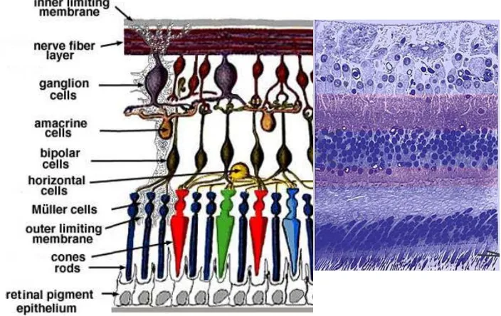
Figure 1.2: Schematic image of the major structures of the lower retina. Image reproduced from [5].
[image:12.612.145.500.375.594.2]There are two types of photoreceptors, defined as rods and cones. Rods are extremely light-sensitive cells responsible for vision in low-light scenarios requiring night vision. Cones are the main cells responsible for daylight vision, less sensitive than cones and with three types differentiated by the three different spectral sensitivities of the cells. The variety of spectral sensitivities of the cones and the lack of color differentiation of the rods are the reasons normal vision is experienced in color but night vision is only in black and white.
High-resolution imaging occurs in the central part of the macular region of the retina, called the fovea. For this region, the cells located above the photoreceptors are thinned and contain no blood vessels. This allows minimal image signal degradation before arriving at the photoreceptors. While for most of the retina, the photoreceptors contain a mixture of rods and cones, the central fovea region contains only a tightly packed region of cones.
The process of converting incoming light into nerve signals in the photoreceptors is accomplished through photosensing pigments called rhodopsin. Disc-shaped lipid membranes containing rhodopsin are packed into the outer segments of the photoreceptors. As the chemical in the discs becomes bleached over the course of a day, the spent photoreceptor outer segment discs must be removed to maintain vision quality [6,7]. Approximately 10% of all outer segment discs are shed each day while the same amount of new discs is produced by the inner segment of the photoreceptors.
Figure 1.3: Schematic of daily phagocytosis process: RPE cells pinching off the used outer segments of photoreceptors while new segments grow in their place.
Figure 1.4: The total lipid content present in the macular region of Bruch’s membrane as a function of the patient age. Data reproduced from [16].
With the decreased metabolism of the RPE cells and the increased blocking of waste passage by Bruch’s membrane, the expected rate of lipids getting stuck to Bruch’s membrane should increase in time. If this rate increases linearly with time, the resulting amount of lipids attached to BM should be an exponential increase over time. Using histological sections of human retinas and analyzing the total lipid content of Bruch’s membrane of the macular region, this trend has been experimentally verified [16]. The rate of lipid deposition on Bruch’s membrane depends on the amount of metabolitic waste passing through the membrane. With the highest density of photoreceptors located within the macular region of the retina (high resolution central vision region), this region accumulates the largest amount of lipids over time.
of these deposits thickens the membrane over the lifetime of patients. Histological measurements of excised retinal tissues have determined a typical thickness change of Bruch’s membrane to more than double over ten decades of patient age [17].
Figure 1.5: Electron micrograph images of Bruch’s membrane with lipids before (left) and after (right) the application of ethanol. Images reproduced from [8].
[image:16.612.113.539.157.366.2]
Figure 1.6: Histology images of normal retina (left) and retina containing thickened Bruch’s membrane (right). Images reproduced from [18].
affected. [19,20] Experiments have demonstrated a measurable drop in the permeability of macromolecules and hydraulic conductivity through Bruch’s membrane as a function of patient age. Limited sampling and variability between human subjects and experimental setups could be a cause for discrepancies to the functional form of the decrease over time (i.e., linear versus exponential decrease with respect to patient age).
Figure 1.7: Decrease of the hydraulic conductivity of Bruch’s membrane over patient age. Data reproduced from [19].
With a decreased supply of oxygen from the choroidal blood vessels as Bruch’s membrane becomes filled with lipids, there is an increased reliance on the retinal blood vessels which lie on top of the retina. These vessels are supplied directly from the optic nerve head, the ocular connection of blood and nerve signals to the rest of the body. Fundus photography takes a picture of the globe of the retina taken through the pupil of the eye. The shadowing of the reflected light due to the major retinal blood vessel absorption can be seen in this type of picture. The foveal region of the retina which produces the highest visual resolution does not have any major blood vessels on the top of the retina.
Figure 1.9: Fundus Photography image of normal healthy eye. The darker image regions demonstrate retinal blood vessel absorption. The fovea is the high-visual-resolution central vision region of the eye and the optic nerve head connects the eye to the rest of the body.
Figure 1.10: Simulated images of normal vision (left) and AMD vision (right). Images reproduced from the National Eye Institute.
In many cases, once the photoreceptors have experienced enough of a decrease of oxygen, the retina will produce signaling to induce creation of new blood vessels to supply more oxygen to this region of the retina. These new blood vessels would extend from the choroid, breaking through Bruch’s membrane in order to feed the retina. This form of the disease is called choroidal neovascularization (CNV), also referred to as wet AMD. VEGF (vascular endothelial growth factor) is a substance made by cells to stimulate the formation of blood vessels, a process called angiogenesis. VEGF was first discovered as occurring in cancerous situations in which blood vessels were created to improve tumor growth [21]. This factor was found to be expressed in human retinas during choroidal neovascularization [22,23,24].
Age-related macular degeneration is classified in three regimes: early, intermediate, and advanced. Early-stage AMD is difficult to identify without professional diagnosis because it occurs without any symptoms or vision loss. Intermediate AMD is the stage where the permeability of Bruch’s membrane has decreased enough that there is a noticeable change in vision of the eye. Since most cases of AMD do not have identical disease progressions in both eyes, patient vision may not notice a change in one eye right away. Advanced AMD is the progression of the disease which can cause severe vision loss. This includes the advanced form of dry AMD as well as wet AMD. There are no early or intermediate stages of wet AMD.
Figure 1.11: Wet AMD produces abnormal blood vessel growth which tries to break through the retinal layers, damaging the retina.
Age Group
Advanced AMD prevalence estimated for age group
Intermediate AMD prevalence estimated in age group
60-69 0.7% (147,000 people in US) 6.4% (1,290,000 people in US)
70-79 2.4% (388,000) 12.0% (1,950,000)
≥80 11.8% (1,080,000) 23.6% (2,160,000)
Figure 1.12: AMD prevalence statistics for the United States [1].
In considering current US statistics of AMD prevalence, about 90% of all classified AMD cases are dry AMD versus wet AMD. But, if only advanced forms of AMD are considered, about 2/3 of cases are wet AMD.
1.2 Current Approaches to Disease Treatment
There are two main approaches in current treatment options for age-related macular degeneration: preventative and stop-gap measures. Preventative treatments attempt to delay the progression of early stage AMD with no vision loss to intermediate and advanced AMD stages where vision loss occurs.
The latest developments on the study of preventative management come from the National Eye Institute supported Age-Related Eye Disease Study (AREDS). AREDS is a 10-year study on the effects of a regimented daily supplement of vitamins and minerals on the progression of AMD for an at-risk patient group already presenting with intermediate stage AMD.
The dietary recommendations come from multiple studies which suggest that while many foods do not seem to have any impact on the progression of AMD, a couple of specific foods have shown very promising results. Consumption of dark leafy green vegetables like spinach, which contain lutein, have demonstrated a decrease in incidences of late stage AMD. Certain types of fish containing omega-3 fatty acids have also shown similar beneficial effects [27].
The NEI has just launched a nationwide study to see if a modified combination of vitamins, minerals, and fish oil can further slow the progression of vision loss from AMD. This new study, called the Age-Related Eye Disease Study 2 (AREDS2), will build upon results from the earlier AREDS study [28].
Stop-gap measures are the only way to describe the treatments for people who are currently suffering from wet AMD. Early treatments of this disease used photodynamic therapy (PDT) to photocoagulate leaking vessels in the eye to prevent future leakage damage from those vessels. To avoid laser damage to the central vision during treatment, only a fraction of wet AMD patients with particular locations of vessels qualified for treatment. Even for the treated patients, within 18 months nearly all had a reoccurrence of wet AMD.
The current popular approach for treatment is to produce drugs which can target the VEGF signaling of the retina. The assumption is that if VEGF was blocked, the retina would not grow any new vessels and wet AMD would not occur. Recent drugs including Avastin (Bevacizumab), Macugen (Pegaptanib), and Lucentis (Ranibizumab) have been designed towards this purpose with varying degrees of success. For all of these type of anti-VEGF drug treatments, there is one consistent trend: Once treatment is stopped, wet AMD progression will continue.
Approximately 1% of patients following a 2-year regiment of eye injections will suffer an infection in the eye as a result. This type of infection generally leads to a complete loss of vision in the eye.
Developments of future treatments will be helped by the diagnostic capabilities of visualizing the disease progression. AREDS was a 10-year study which had effectiveness determined by visual acuity measurements. With the ability to measure the more subtle changes associated with the transitions in AMD, the effectiveness of treatments can be determined in shorter times and adjustments can be made to ineffective treatment regimes for patients.
1.3 Current Diagnostic Technologies and Limitations
AMD treatments are partly limited by the availability of diagnostic technologies able to screen the general population for disease management. An ideal screening tool for AMD needs to be able to:
a) Identify the earliest stages of AMD before patient has visual symptoms so that preventative treatments can be applied
b) Identify the earliest transitions from dry AMD to wet AMD to improve the efficiency of treatments directed towards wet AMD
c) Monitor quantitative changes of disease progression and treatment efficacy to improve future disease treatments
There are many technologies currently in use for diagnostic purposes for ocular exams. Each has its own benefits and limitations that need to be discussed in order to determine which one has the greatest potential of being the primary screening diagnostic for AMD.
1.3.1 Histology
[image:24.612.149.501.390.612.2]Histology has always been a valuable tool for understanding tissue morphology over the course of a disease progression. Most of the structural models of the retina have been developed through study of the excised retinal tissues using optical microscopy. Histological staining combined with microscopy adds an additional level of contrast for improved visualization at a very high resolution. Unfortunately, biopsy of the retina to get the excised tissue would have a severe negative impact on the vision of any living eye so this technique is limited to post-mortem subjects only. Monitoring progress of a disease within one individual is not possible with this method.
1.3.2 Visual Acuity
Visual acuity is a coarse measurement of the sharpness of the retinal focus within the eye. It is the standard measurement used by optometrists to determine prescriptions for glasses. Used in AMD diagnostics, visual acuity has been used to determine wet AMD drug effectiveness. As sub-retinal fluid accumulates in wet AMD, the lifting of the retina causes a change in the patient’s visual acuity.
[image:25.612.254.391.414.605.2]There are two main issues with using visual acuity as the main diagnostic measurement [29]. First, as a coarse measurement of the mean visual acuity over the fovea, visual acuity is not designed to quantify very small localized changes due to disease progression [30]. Large visual acuity drops measured with this method correspond very well with the progression of the disease. Improvements of visual acuity measured over time for a patient could correspond to an improvement of the disease progression. They could just as easily be explained by a patient adapting to their current vision or adapting to the test itself. Without additional diagnostics, it would be difficult to discern the true scenario.
1.3.3 Amsler Grid
The Amsler grid is a simple grid composed of horizontal and vertical lines with a dot in the center. When a patient focuses on the dot and observes any of the lines as distorted or missing, this might identify the existence of locations of sub-retinal fluid associated with a leak from choroidal neovascularization.
Figure 1.15: Amsler grid viewed under normal vision versus simulated wet AMD leak.
This test is user-based and very qualitative, making it a poor diagnostic tool by itself. The Amsler grid is ideal for directing to an eye care professional potential wet AMD patients who otherwise may not have gotten an examination until much later in the progression of the disease.
1.3.4 Fundus Photography
Early stages of dry AMD are roughly linked to the appearance of localized fatty deposits called drusen. By identifying the color, size, and number of drusen which appear on the fundus image, the early stage of AMD can be classified. Fundus photography is capable of visualizing many aspects of AMD progression including pigment abnormalities, regional cell death in the retina (called geographic atrophy), and choroidal neovascularization (CNV). With blood contrast occurring due to the regional light absorption for the image, the earliest stages of CNV may experience limited contrast in this technique.
Figure 1.16: Fundus photography images for AMD eyes. Drusen deposits in the fovea region are associated with dry AMD (left) and observed blood vessel leaks are caused by wet AMD (right). Images reproduced from [8].
Fundus photography has a lot of characteristics that make it ideal as a screening tool: It is quick, easy, risk-free, and relatively comfortable for patients. Until the relationship between the drusen observed in AMD patients and the progression of the disease can be understood, this technique will remain a qualitative measure for early AMD diagnostics. With absorption as the main blood contrast observed, the earliest stages of wet AMD will remain very difficult to discern.
1.3.5 Fluorescein Angiography
system. Fluorescein is a molecule which will fluoresce green at a wavelength around 521 nm while undergoing absorption of blue light at a wavelength around 494 nm. Fundus photography with blue light illumination and a green filter on the camera will allow visualization of the fluorescein as it circulates through the retinal vasculature.
Figure 1.17: Fluorescein angiography images taken at different time points after dye injection. The time sequence of stages are the arterial stage (upper left), the venous stage (upper right), the mid phase (lower left), and the late phase (lower right).
(ICGA) allows improved visualization of the deeper choroidal blood vessels as well as the retinal vessels.
The injections required for this technique limit the general screening capabilities of this technique. Possible adverse reactions to injections or to the fluorescein sodium solution used are the main concerns with this method [32,33]. If the diagnostic capabilities of the angiography techniques were possible without the injections, it would be an ideal screening tool for identifying the earliest stages of wet AMD.
1.3.6 Ultrasound
Ultrasound uses sound waves to identify interfaces within the sample. Each depth reflection is separated from each other by the differing travel times of the sound waves reflecting back to the detector. Typical high-resolution ultrasound is capable of separating distinct layers 20 microns from each other. To allow the sound waves to propagate to the retina, the sound wave transducer must be placed in physical contact on the eye which may not be comfortable for all patients. Ultrasound is commonly used to assess the retina for cases with dense cataracts which limit the optical accessibility of the retina. Optical imaging is generally preferable to ultrasound as a screening instrument.
1.3.7 Scanning Laser Ophthalmoscope
The major limitation to optically image the retina depends on the optical properties of the eye. With the sclera considered optically opaque, the retina is accessible by imaging through the cornea and lens of the eye. The aqueous humor is the fluid which fills the globe of the eye between the lens and the retina, which optically can be considered as water. The absorption profile of water limits the available wavelengths to use for retinal imaging.
absorption of the light in these cases limit the usefulness of certain wavelength ranges of illumination light sources.
[image:30.612.219.426.297.510.2]The scanning laser ophthalmoscope (SLO) performs confocal microscopy imaging of the retina, using the lens of the eye as the focusing element. By scanning a laser transversely across the retina and measuring the reflected light, an image comparable to fundus photography is created. In this system, the image is created from monochromatic laser light. Through the appropriate selection of laser wavelength and illumination power levels, image contrast can be adjusted with a higher level of flexibility than standard fundus photography [34].
Figure 1.18: Wavelength absorption spectra of water. Horizontal line corresponds to absorption of 0.2 cm-1.
1.3.8 Optical Coherence Tomography
than the speed of sound in tissue, it is technologically challenging to temporally separate out the reflections. Instead of pushing technology to attempt to distinguish femtosecond temporal resolution, an interferometric technique was developed which allows the separation of retinal layers through spatial discrimination.
OCT is sometimes considered in vivo optical histology because it is capable of producing 3D structural information of a sample. The most popular OCT retinal imaging system (Stratus OCT, created by Carl Zeiss Meditec) demonstrates a depth resolution in retinal images of 10 µm in tissue [35]. While it is has not reached the resolution level of current histology imaging capabilities, this technique creates images which correlate to expected histological measurements.
Figure 1.19: Schematic image of retina with the retinal layers identified. Image reproduced from reference [34].
Figure 1.20: OCT Image acquired with Carl Zeiss Meditec Stratus OCT system, with labeling of identified retinal layers. The structure is consistent with the expected layering of the schematic of the retina in Figure 1.19. Image reproduced from [34].
1.3.9 Summary of Diagnostic Technologies
Optical imaging techniques are very capable as a quick and risk-free screening tool for patients. For AMD diagnostics, fundus photography and fluorescein angiography are currently the most valuable diagnostic tools available. The diagnostic capabilities would be enhanced further with additional quantitative information of the fundus images as well as the possibility of achieving fluorescein angiography images without requiring the dye injection.
1.4 References
1. “Prevelance of Blindness data tables–Based on Archives of Ophthalmology, Volume 122, April 2004 Data,” National Eye Institute,
http://www.nei.nih.gov/eyedata/pbd_tables.asp.
2. N. Congdon et al., “Causes and prevalence of visual impairment among adults in the United States,” Arch. Ophthalmol. 122, 477 (2004).
3. “65+ in the United States: 2005–Current Population Reports,”
http://www.census.gov/prod/2006pubs/p23-209.pdf.
4. “Defining the Prevalence of AMD and Investigating Racial Differences,” Retina Today, January/February 2007,
http://www.retinatoday.com/Html%20Pages/0107/RT0107_cover_bressler.html. 5. “Simple anatomy of the retina,” Webvision, http://webvision.med.utah.edu/sretina.html. 6. R.W. Young, “The renewal of photoreceptor cell outer segments,” J. Cell Biol. 33, 61
(1967).
7. R.W. Young et al., “The renewal of rod and cone outer segments in the rhesus monkey,” J. Cell Biol. 49, 303 (1971).
8. S.E. Fraser, “New Sight for Old Eyes,” California Institute of Technology Engineering and Science Magazine 64, 3 (2006).
9. R.W Young et al., “Participation of the retinal pigment epithelium in the rod outer segment renewal process,” J. Cell Biol. 42, 392 (1969).
10. M.M. LaVail et al., “Rod outer segment disk shedding in rat retina: relationship to cyclic lighting,” Science 194,1071 (1976).
11. R.W. Young et al., “The daily rhythm of shedding and degradation of cone outer segment membranes in the lizard retina,” J. Ultrastruct. Res. 61,172 (1977).
12. M.J. Hollenberg et al., “The fine structure of Bruch's membrane in the human eye,” Can J. Ophthalmol. 4, 296 (1969).
13. F. Emeline et al., “Loss of Synchronized Retinal Phagocytosis and Age-related Blindness in Mice Lacking αvß5 Integrin,” J. Exp. Medicine 200, 1539 (2004). 14. L. Feeney, “Lipofuscin and melanin of human retinal pigment epithelium.
Fluorescence, enzyme cytochemical, and ultrastructural studies,” Invest. Ophthalmol. Vis. Sci. 17, 583 (1978).
15. L. Feeney-Burns et al., “The fate of the phagosome: conversion to ‘age pigment’ and impact in human retinal pigment epithelium,” Trans. Ophthalmol. Soc. U.K. 103, 416 (1983).
16. F. G. Holz et al., “Analysis of lipid deposits extracted from human macular and peripheral Bruch's membrane,” Arch. Ophthalmol. 112, 402 (1994)
17. R.S. Ramrattan et al., “Morphometric analysis of Bruch's membrane, the
choriocapillaris, and the choroid in aging,” Invest. Ophthalmol. Vis. Sci. 35, 2857 (1994).
18. W.R. Green and C. Enger, “Age-related Macular Degeneration Histopathologic Studies: The 1992 Zimmerman Lorenz Lecture,” Ophthalmology 100, 1519 (1993). 19. C. Starita et al., “Hydrodynamics of Ageing Bruch's Membrane: Implications for
20. D.J. Moore et al., “The Effect of Age on The Macromolecular Permeability of Human’s Bruch’s Membrane,” Invest. Ophthalmol. Vis. Sci. 42, 2970 (2001).
21. D.R. Senger et al., “Tumor cells secrete a vascular permeability factor that promotes accumulation of ascites fluid,” Science 219, 983 (1983).
22. M.D. Sternfeld et al., “Cultured human retinal pigment epithelial cells express basic fibroblast growth factor and its receptor,” Curr. Eye Res. 8, 1029 (1989).
23. A.P. Adamis et al., “Synthesis and secretion of vascular permeability factor/vascular endothelial growth factor by human retinal pigment epithelial cells,” Biochem. Biophys. Res. Commun. 193, 631 (1993).
24. A. Kvanta, “Expression and regulation of vascular endothelial growth factor in choroidal fibroblasts,” Curr. Eye Res. 14, 1015 (1995).
25. Macular Degeneration International: The Foundation Fighting Blindness,
http://www.maculardegeneration.org/agedex.html.
26. “Laser Treatment Does Not Prevent Vision Loss For People With Early Age-Related Macular Degeneration,” US Environmental Protection Agency,
http://www.epa.gov/aging/press/othernews/2006/2006_1101_ons_1.htm. 27. “Age-related Macular Degeneration: What you should know,” NEI Publication,
http://www.nei.nih.gov/health/maculardegen/webAMD.pdf .
28. “Age-Related Eye Disease Study 2 (AREDS2),” https://web.emmes.com/study/areds2/. 29. “The importance of Vision-Related Quality of Life in Patients Treated with
Neovascular AMD,” Retina Today, January/February 2007,
http://www.retinatoday.com/Html%20Pages/0107/RT0107_medical_chang.html. 30. “Visual Acuity,” Wikipedia, http://en.wikipedia.org/wiki/Visual_acuity.
31. S.O. Sykes et al., “Detecting recurrent choroidal neovascularization. Comparison of clinical examination with and without fluorescein angiography,” Arch. Ophthalmology 112, 1561 (1994).
32. L. Yannuzzi et al., “Fluorescein angiography complication survey,” Ophthalmology 93, 611 (1986).
33. M. Hope-Ross et al., “Adverse reactions to indocyanine green,” Ophthalmology 101, 529 (1994).
34. P.F. Sharp et al., “The scanning laser ophthalmoscope,” Phys. Med. Biol. 42, 951 (1997).
35. “Stratus OCT TM: Real Answers in Real Time,” Brochure from Carl Zeiss Meditec,
C h a p t e r 2
OPTICAL COHERENCE TOMOGRAPHY
Through the understanding of optical coherence tomography (OCT), the fundamental limits of imaging performance can be identified. Within these limits functionality improvements can be identified to move beyond the capabilities of currently available OCT systems. It is important to determine the ability of OCT to adapt towards quantitative diagnostics for AMD progression.
2.1 Basics of Optical Coherence Tomography (OCT)
2.1.1 Michelson Interferometer with Single Wavelength Light Source
Optical coherence tomography is based upon a Michelson interferometer configuration. Consider a single wavelength narrow bandwidth laser source incident on a Michelson interferometer. The incoming light is split using a beamsplitter into two interferometer arms, designated as the reference and sample arms. The light is reflected back through the beamsplitter to be collected by the photodetector, which converts the measured power into an electrical current.
Looking at the complex form of the electric field of the laser light, the light traveling through the reference arm of the interferometer arrives at the detector has the form of
)) (
exp( ~
0 , +ϕ
= R totalR R E i kz
E , where ztotal,R = z1+2zR +z4 is the total optical path the light
has traveled through the interferometer, ϕ0 is phase of electric field of light source before it
enters the interferometer, and k=2π/λ for the light source of wavelength λ. Similarly, the electric field traveling through the sample arm of the interferometer is of the form
)) (
exp( ~
0 , +ϕ
= S totalS S E i kz
E , where ztotal,S =z1+2zS +z4 is the total optical path traveled
Figure 2.1: Free space Michelson interferometer with single reflector in each arm, designated as reference and sample.
The photodetector measures intensity of light, calculated by the magnitude of the total electric field arriving at the detector.
2 0 , 0
, 2
)) (
exp( ))
( exp( ~
~ + = +ϕ + +ϕ
= S R S totalS R totalR
Detector E E E i kz E i kz
I
= ES2 +ER2 +2ESERcos(kztotal,S +ϕ0 −kztotal,R −ϕ0)
=ES2 +ER2 +2ESERcos(2k(zS −zR))
=IS +IR+2 ISIR cos(2k(zS −zR))=IDetector(k,zS −zR) (2.1)
where ~ 2 2
S S
S E E
I = = and IR = E~R 2 =ER2.
2.1.2 Michelson with Broad Bandwidth Light Source
For a broad bandwidth light source, treat each wavelength component as an individual light source which does not interfere with any other wavelength than itself. Define
and , where S(k) is normalized spectral function of the light
source, and R ) (
0S k
I R
IR = R IS =RSI0S(k)
a is percentage of original light intensity I0 reaching the detector for light
traveling through arm a. Assuming uniform efficiency of the detector over the light source spectra, the detector measures the sum of all light source contributions for all wavelengths. Calculating in terms of k-space:
I z z I k z z dk
k
R S Detector R
S − )=
∫
( , − )(
R I R I S k R R I S k k z z dk
k R S R S R S
∫
+ + −= (( 0 0) ( ) 2 0 ( )cos(2 ( )))
R R I R R I S k k z z dk
k R S R S R
S + +
∫
−=( ) 0 2 0 ( )cos(2 ( )) . (2.2)
The function is an autocorrelation of the light source spectra
that is defined as the Weiner-Khinchin theorem (Fourier transform of the magnitude of the electric field). The coherence function, which will be defined as and is centered
around z = z
dk z z k k S k R S
∫
( )cos(2 ( − )))) (z fC
S - zR, is a function which determines the effect on the interference signal when
reflections from the two arms of the interferometer are not of equal path length.
The coherence length is the quantitative metric of the spatial extent each interference
reflection is measured over. This is defined as the full width half-maximum (FWHM) of the envelope of the spatial measurement of the coherence function. The coherence length describes the ability of the system to separate different interference reflections from each other.
C
0
D
e
te
c
to
r In
te
n
s
ity
zR-zS
0
Coherence Length l
c
D
e
te
ct
or
I
n
tensi
ty
zR-zS
Figure 2.2: Measured light intensity at output of the Michelson interferometer as a function of the difference of the optical path lengths from the interferometer arms for the cases of single wavelength light (left) and broad bandwidth light (right). The full width half maximum (FWHM) of the interference fringe maximum is labeled as the coherence length.
2.1.3 Comparing Reflectivity to Interferometer Detector Signal
Consider the Michelson interferometer setup with a layered structure in the sample arm instead of a single reflector. The interference signal measured is the coherence function convoluted with the reflectivity profile of the sample.
R
e
fl
e
c
tiv
ity
zR-zS
D
e
te
c
tor Intensity
zR-zS
2.2 Axial Resolution
The ability to separate fringes from reflections of different depths depends on the shape of the coherence function, which relies on the light source properties. This depth separation is referred to as the axial resolution. Consider the extreme cases:
a) For an infinitely narrow light source spectrum such that S(k)= S0δ(k0),
) (z
fC = ( )cos(2 ( ))) cos(2 0( S R))). (2.3) k
R
S z dk k z z
z k k
S − ∝ −
∫
In this case, interference fringes are observed for all zS −zR values. All reflections from
every depth within the same are observed all at the same time, resulting in the measurements being dominated by the strongest reflection.
b) For an infinitely broadband light source such that S(k)=1 for all k,
) (z
fC = ( )cos(2 ( ))) ( S R). (2.4) k
R
S z dk z z
z k k
S − ∝ −
∫
δFor this case, no interference would be observed unless the interferometer arms were of identical optical path lengths.
Spectral Shape and Coherence Function Tradeoffs
A finite-width broad bandwidth light source will measure interference over a spatial extent
determined by the light source properties. The coherence function contains the
oscillatory interference fringe function based on the center wavelength of the light source combined with an envelope function which defines the spatial extent of the interference measurement. The coherence length can be considered as the axial resolution, which
determines the minimum depth difference at which two identical distinct reflections can be differentiated from each other.
) (z fC
C
For a Gaussian source spectra where the interferometer arm length difference is defined
, the coherence function can be calculated using the
light source spectral form S(k) = S
R S z
z
z= − f z S k kz dk
k
C( )=
∫
( )cos(2 )0 exp(-4 ln 2 (k-k0)2/∆kFWHM2), where the spectrum is
centered around k0=2π/λ0 and λ0 is the center wavelength of the light source:
⎟ ⎟ ⎠ ⎞ ⎜ ⎜ ⎝ ⎛ =
=
∫
S k kz dk∫
S k i kz dkz f
k k
C( ) ( )cos(2 ) Re ( )exp( 2 )
⎟ ⎟ ⎠ ⎞ ⎜ ⎜ ⎝ ⎛
=Re exp( 2 )
∫
( ')exp( 2 ' ) ''
0z S k i k z dk
k i
k
. (2.5)
Using ( ') exp( ( ')2), where
0 C k
S k
S = − k'=k−k0 and C=4ln2/∆kFWHM2:
⎟ ⎟ ⎠ ⎞ ⎜ ⎜ ⎝ ⎛ −
=Re exp( 2 )
∫
exp( ' )exp( 2 ' ) ' )(
'
2 0
0 i k z Ck i k z dk
S z
f
k C
Re
(
exp( 2 )exp( 2/ ))
0
0 i k z z C
f − = ) 2 ln 4 / exp( ) 2
cos( 0 2 2
0 k z k z
f −∆ FWHM
= . (2.6)
In this case, the envelope function is a Gaussian function with a full width half maximum (FWHM) of ∆zFWHM =4ln2/∆kFWHM =lC. Defining the coherence length in terms of
wavelength uses C l FWHM FWHM k λ λ
π ⎟∆
⎠ ⎞ ⎜ ⎝ ⎛ = ∆ 2 0
2 to calculate:
FWHM FWHM C l λ λ λ λ
π ∆ = ∆
= 02
2
0 0.44
2 ln 2
. (2.7)
For the given light source bandwidth from the above equation, maximizing FWHM of the light source should produce the best axial resolution. Consider a top-hat spectra centered
∫
∫
+∆ ∆ − = = 2 / 2 / 0 0 0 ) 2 cos( ) 2 cos( ) ( ) ( FWHM FWHM k k k k kC z S k kz dk S kz dk
f z k z k z k f FWHM FWHM ∆ ∆
= 0cos(2 0 )sin( ), (2.8)
which leads to a coherence length of:
FWHM FWHM C k l λ λ ∆ = ∆
= 3.79 0.60 02 . (2.9)
To compare these coherence length calculations directly, consider the case of the top-hat spectrum and the Gaussian spectrum with similar spectral extent such that
FWHM Gaussian
FWHM Tophat
FWHM λ λ
λ = ∆ = ∆
∆ , 2 , 2 , as shown in Figure 2.4.
[image:41.612.188.461.348.556.2]
In
te
n
s
ity
Wavelength
Figure 2.4: Plots of Gaussian (red) and top-hat (blue) spectral functions for the case of ∆λFWHM,Tophat = 2∆λFWHM,Gaussian
= 2∆λFWHM.
In this case, the top-hat source coherence function is
FWHM Tophat C l λ λ ∆ = 02
, 0.30 , and the
Gaussian source coherence function is 0.44 1.47( , )
2 0
, CTophat
The coherence length cannot be considered as the only important factor to consider.
With the typical sample containing reflections that vary over several orders of magnitude, the spatial form of the coherence function determines how the weaker reflections are identified when located close to a strong reflection. If all of the reflections were identical within a sample, this would not be a consideration.
C
l
The interference signal in OCT is defined by the magnitude of the envelope of the coherence function convoluted with the reflectivity profile of the sample over depth. So for a normalized OCT signal of a given reflector, the coherence length is defined by the width, defined by the -6dB points (as opposed to the -3dB points used for the FWHM of the coherence envelope). On a linear scale, the side lobe variations of the coherence function due to the top-hat spectra do not seem to have much of an effect. On a logarithmic scale, the side lobes of this function are significant and extend out spatially far beyond the coherence length. On this scale, the coherence function of the Gaussian source spectra can be seen to have a larger coherence length but without any side lobes.
0 0.0
0.2 0.4 0.6 0.8 1.0
N
o
rm
al
iz
ed OCT
Si
gn
al
zR-zS
0 1E-4
1E-3 0.01 0.1 1
y
zR-zS
These two cases demonstrate the tradeoffs between coherence function shape and coherence length for a given source spectrum. The top-hat spectrum was the largest spectral FWHM for a given spectral width. The coherence length minimum for this given spectral width was at the tradeoff for the side lobes of the function. The coherence function created from the Gaussian spectra contains no side lobes, but has a relatively larger coherence length. Spectral shaping of the light spectrum allows adjustments between the coherence length and side lobes of the coherence function.
As illumination spectral widths become wider, dispersion compensation becomes more important. Dispersion mismatch between the interferometer arms causes a reflection to appear at different optical depths for different wavelength components of the light source, effectively broadening the coherence function and increasing the coherence length.
2.3 Acquiring Fringe Data to Create OCT Images
Optical coherence tomography (OCT) is the method of imaging which plots the spatial distribution of the envelope of interference fringes from a broad bandwidth light source in a Michelson interferometer configuration. The main question is: How is the envelope of the interference fringes determined?
For a single photodetector power measurement of an interference fringe, the measurement is of the form:
P(zS −zR)=PDC +PINT fC(zS −zR)
))) (
2 cos( )
( S R 0 S R
E INT
DC P f z z k z z
P + − −
= . (2.10)
DC
P is the sum of all the powers measured by the photodetector, is the maximum
power of the interference fringe, and is the envelope function portion of the
coherence function, normalized to a maximum of 1. The quantity of interest is
, which is the non-normalized envelope function. The difficulty in
INT
P
) (z fE
)
( S R
E
INT f z z
determining this factor from one detector measurement is due to two additional unknown
variables beyond the quantity of interest: PDC and zS −zR.
z
R-zS
Det
e
ct
or
Power
Figure 2.6: Schematic illustrating the lack of information for using a single point measurement to measure the interference fringe intensity.
The interferometric portion of the signal cos(2k0(zS −zR))is very sensitive to the relative
position of the two reflections. It is easier to consider this signal in terms of the
relative phase
R
S z
z −
R
S φ
φ − of the interference fringe because, while the envelope function
is sensitive to distance changes on the order of microns, the fringe oscillation
is sensitive to changes on the order of nanometers (1000 times more
sensitive). )
( S R
E z z
f −
)) (
2
cos( k0 zS −zR
The relative phase of the interferometer φS −φR is defined as 4π(zS −zR)/λ0, so any
relative motion in the system with a magnitude of at least λ0/2 will see a full oscillation in
Det
e
ct
or
Power
zR-zS
Figure 2.7: Schematic image of an interference fringe sampled using a small interferometer path length change.
There are several methods to sample the interference fringes to produce an OCT image. The most commonly used method utilizes a linear scan of the reference arm path length to sample all of the interference fringes over the entire depth of the sample. Keeping consistent with ultrasound scan terminology, a single scan along the depth of the sample is called an A-scan. Creating a two dimensional reflectance image through multiple A-scans over a range of transverse locations is called a B-scan.
As a screening tool for the retina, there is an additional interest in flexibility of the scan directions. Transverse images, also called en face images or C-scans, allow imaging at one depth of the interference fringes over the entire plane of the retina. If the primary acquisition of OCT data is through A-scans, the only way an en face image could be created would be through a 3D data set composed of A-scans measured over all transverse locations of interest. With mechanical scanning technologies limiting the maximum A-scan rate in TDOCT, it is not practical to produce transverse images this way.
Transverse scans followed by transverse scans in the perpendicular direction would produce C-scans. En face images are ideal in retinal imaging to screen an entire retina for signs of a disease, but allowing for it to occur at a single tissue depth of interest.
To acquire fringe information to allow for transverse scanning as the primary scan direction, the interference fringes must be sampled. The easiest way to sample requires changes in the relative optical path length much smaller than the axial resolution, which has numerous options available for creating small phase changes in the system at high speeds to measure the fringes [3-7].
2.4 SNR of Time Domain OCT
In TDOCT, the interferometric signal is measured as a current by the photodetector. Looking at the maximum fringe signal, the interferometer current i(zS −zR) is given by:
)) ( 2 cos( ' 2 ) ( 0 R S S R R
S k z z
h P P z
z
i − = −
ν η
(2.11)
where η' is the quantum efficiency of the photodetector to convert photons to electrons.
are the powers arriving at the detector from the reference and sample arms of the
interferometer, respectively and
S R P
P ,
0 ν
h is the average energy of the photon from the light
source.
The signal in OCT is the spatial average of the square of the interferometer current
over several fringes:
2 I(z) 2 0 2 2 2 ) ( ' 2 ) ( I(z) ν η h P P z
i R S
z =
= . (2.12)
2 noise 2/
I(z)
SNR= σ . (2.13)
There are three types of noise sources occurring over time τ’ acquisition of a given pixel in the TDOCT acquisition: detector noise, shot noise, and relative intensity noise (which is also referred to as excess noise). The total noise in OCT is determined by the summation of the variance of all three types of noise sources:
2 excess 2 shot 2 detector 2
noise σ σ σ
σ = + + . (2.14)
The detector noise can be considered a constant source of noise, independent of the amount of power incident on the detector.
constant
2 detector =
σ (2.15)
Shot noise is defined by the statistical fluctuations which occur for the measure of a finite number of particles in a detector over a given amount of time. For electrical currents, the expected probability distribution for the number of electrons during the acquisition of the detector is given by a Poissonian distribution around the expected mean number of electrons. For this distribution, the variance of the measured electrons is equal to the mean
number electrons measured within the time τ’ of the detector, which is determined from the total power incident on the detector. For the case of , which is applicable for most
OCT imaging scenarios, the shot noise variance is given by:
S R P P >> ' ) ( ' ' ) ( ) ( ' 0 0 2 τ ν η τ ν η σ h P h P
PR S R
shot ≈
+
= . (2.16)
Relative intensity noise (RIN) describes the optical intensity fluctuation noise of the light source [8]. With the same assumption of PR >>PS:
' ' ' ) ( ' 2 0 2 0 2 τ τ ν η τ τ ν η
σ R S coh R coh
excess h P h P P ⎟⎟ ⎠ ⎞ ⎜⎜ ⎝ ⎛ ≈ ⎟⎟ ⎠ ⎞ ⎜⎜ ⎝ ⎛ +
In this equation τcoh is the coherence time, defined by FWHM coh c λ λ π τ ∆ ⎟ ⎠ ⎞ ⎜ ⎝ ⎛
= 02 2 / 1 2 ln 2
, where c
is the speed of light, λ0 is the center wavelength, and ∆λFWHM is the bandwidth of the light
source.
Each of the different noise sources dominate in different regimes, which are determined by the total incident power on the detector, which is approximately described by PR. From the
properties of the individual noise sources and the OCT signal dependence on PR, the ideal
SNR performance would occur in the regime where the shot noise dominated the noise sources.
For the ideal SNR shot-noise limited case, given a TDOCT pixel acquisition time τ’:
SNRTDOCT ) ( ' ' 2 ' ) /( ' ) /( ' 2 0 0 2 0 2 ν τ η τ ν η ν η h P h P h P P S R S R =
= . (2.18)
2.5 Spectral Domain Optical Coherence Tomography (SDOCT)
Time domain optical coherence tomography (TDOCT) measures the interference in the case where a sample reflection has the same optical path length as the reference reflection. By measuring all of the interference fringes from all wavelength components at the same time within a photodetector, all of the non-equal path length fringes are rejected through destructive interference with each other.
The interference fringes have the form of cos(2k(zS −zR))for a given optical path
difference of the interferometer arms of zS −zR. Measuring the interference fringes in
There are two different methods which fall under the category of FDOCT. The first method measures the interference fringes in k-space using a spectrometer to separate the wavelength components for measurement. This technique is called spectral domain optical coherence tomography (SDOCT) [10,11]. The other method utilizes a swept source laser with a narrow-band instantaneous spectral line width in the interferometer to vary the wavelength over time to be measured by a photodetector. This technique is referred to as swept source optical coherence tomography (SSOCT) or optical frequency domain imaging (OFDI) [12,13]. Regardless of the FDOCT method chosen, the calculation of the OCT signal from the spectral information remains the same.
Power measured in k-space for sample reflections (labeled by j, sample path locations zj
=2(zSj −zR) with reflected power labeled as PSj:
∑
∑
+ + = j j Sj R j SjR k P k P k P k kz
P k
P( ) ( ) ( ) 2 ( ) ( )cos( )
∑
≠ − + j ij i j i SjSi k P k k z z
P , )) ( cos( ) ( ) ( 2 2 1
. (2.19)
For most scenarios PSj << PR which allows the last term to be ignored. By removing the DC
component of the measured power signal ~ PR (k), we are left with the approximate
summation of all the sample reflections interfering with the reference reflection.
∑
≈ − j j Sj RR k P k P k kz
P k
P( ) ( ) 2 ( ) ( )cos( )
∑
≈j
j Sj
RP S k kz
P ( )cos( )
2 (2.20)
dk ikz kz k S P P k P k P FT j j Sj R
R( )) 2 ( )cos( )exp( )
) ( (
∑
∫
∞ ∞ − ≈− . (2.21)
With the assumption that S(k) changes slowly relative to , and making the
assumption that z
) cos(kzj
j=2(zSj −zR) 0 simplifies the equation to: ≥
dk z z ik k S P P k P k P FT z I j j Sj R
R( )) ( )exp( ( ))
) ( ( ) ( ~ = − ≈
∑
−∫
∞ ∞ − ) ( ~ j C j SjRP f z z
P −
=
∑
. (2.22)) ( ~
j C z z
f − is the complex form of the coherence function derived earlier in this chapter
such that Real[~fC(z−zj)]= fC(z−zj)and the amplitude of this function is the definition of
the envelope of the coherence function. The signal in OCT is the magnitude of the Fourier transform of the interference signal in k-space:
2 2 2 ) ( ~ )) ( ) ( ( ) ( ~ j C j Sj R
R k P P f z z
P k P FT z
I = − ≈
∑
− . (2.23)The result is a summation of the magnitude of the envelope of the coherence functions centered around each of the sample reflection locations zj =2( ), weighted by the
power collected from each of the reflections P
R Sj z
z −
Sj. This is identical to the form of the OCT
signal measured in TDOCT.
One option available to SDOCT is the ability to adjust the coherence function through numerical spectral shaping. With the direct measurement of the spectral interference fringes, numerical shaping of the fringes before the Fourier transform is performed can
alter the shape of the coherence function and improve the coherence length while
suppressing the side lobes.
For retinal imaging, the ideal method of FDOCT is not easy to determine. Only recently has there been developments of fast swept source lasers centered at wavelengths capable of retinal imaging (1300 nm light is absorbed too much while propagating through the 5cm of aqueous humor of the eye) [14,15,16]. High-speed line scan CCD cameras are readily available for incorporation into a spectrometer design [17,18,19]. For the extent of this project, SDOCT is chosen as the FDOCT method used for retinal imaging.
2.6 SNR of SDOCT
Define spectral domain optical coherence tomography (SDOCT) system, where the power from the reference arm arriving at the spectrometer is PR and power from the sample arm
arriving at the spectrometer is PS. Assume that PS << PR. Integration time of the
spectrometer is τ. The spectrometer has M pixels used in k-space measurements. Assume shot-noise-limited performance of the SDOCT system.
Number of electrons on CCD pixel in k-space:
∑
+ + + = j DC Sj jj k kz F k N k
S k
F( ) 2 ( )cos( φ ) ( ) ( ). (2.24)
) (k
Sj is the interferometric signal is defined as Sj(k)=η PR(k)PS(k)Rjτ/hν0 for a sample
reflection Rj at optical path difference zj =2(zSj −zR) of interferometer. The summation of
this signal is taken over all of the sample reflections. Define =
∑
kR
R P k
P ( ), =
∑
k S
S P k
P ( ).
) ( ) (k N k
FDC + is the shot noise distribution of electrons. The mean number of electrons
is given by
) (k
FDC ηPR(k)τ/hν0, where η is the combined light collection and electron
conversion efficiency of the spectrometer for photons of energy hν0. is the random
portion of the Gaussian distribution with variance and zero mean.
) (k N 0 ) (
2 η ( )τ/ ν
σ N k = PR k h
![Figure 1.2: Schematic image of the major structures of the lower retina. Image reproduced from [5]](https://thumb-us.123doks.com/thumbv2/123dok_us/8593319.864002/12.612.144.511.83.301/figure-schematic-image-major-structures-retina-image-reproduced.webp)