Mobile robot Navigation Techniques: A Survey

Mobile robot Navigation Techniques: A Survey

Vikas Verma

1

1Jaipur National University, jagatpura, Jaipur [email protected]

Abstract: This paper describes the developments of different basic techniques for mobile robot navigation during the last 10 years.Now a day’s

mobile robots are vastly used in many industries for performing different activities. Controlling a robot is generally done using a remote control, which can control the robot to a fixed distance, we discuss three basic techniques for mobile robot navigation the first technique is the combination of neural network and Fuzzy logic makes a neuro fuzzy approach. Second method is the Radio frequency technique which is control system for a robot such that the mobile robot is controlled using mobile and wireless RF communication. Third method is robot navigation using a sensor network embedded in the environment. Sensor nodes act as signposts for the robot to follow, thus obviating the need for a map or localization on the part of the robot. Navigation directions are computed within the network (not on the robot) using value iteration.

Keywords: Fuzzy logic, neural network, Radio frequency, signposts

1.

In the field of industrial and service robotics, the problem of wheel-based mobile robot navigation has attracted considerable attention in the recent years. Solution techniques to this complex problem involve handling many issues including among the others acquisition and processing of sensory data, decision making, trajectory planning, and motion control.

From the motion control point of view, one major problem is the development of good and robust trajectory tracking algorithms in a variety that must also cover the many different types of mobile robots. In fact, various mobility configurations can be found depending, e.g., on the number and type of the wheels, their actuation, the single- or multibody vehicle structure, etc.

Main issue in mobile robot is navigation in an uncertain and complex environment and considerable research has been done for making an efficient algorithm for the mobile robot navigation. Among them, adaptive control and behavior based control are most popular control algorithms and driving research in robot navigation. Adaptive navigation control is a method using pre-defined equations that represent the robot’s moving path to reach targets and show strong ability in well-known environment [1]. However it is hard to build precise path generating equation for unknown and complex environment. Evolutionary computation provides an alternative

knowledge description by means of linguistic mathematical or logical models. Fuzzy control provides a flexible tool to model the relationship between input information and control output and is distinguished by its robustness with respect to noise and variation of system parameters. Soft computing is concerned with the design of intelligent and robust systems, which exploit the tolerance for imprecision inherent in many real world problems. In order to achieve this objective, soft computing suggests fuzzy logic reasoning.

The other popular Technique for Controlling a robot is generally done using a remote control, which can control the robot to a fixed distance, but here by designing control system for a robot such that the mobile robot is controlled using mobile and wireless RF communication. In this method controlling is done depending on the feedback provided by the sensor. This contains different modules such as

 Wireless unit module

 Sensing and controlling module

successfully decide which node neighborhood it belonged to. Extensive experiments with a robot and a sensor network confirm the validity of the approach.

2.

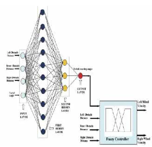
The neural network used is a four-layer perception. This number of layers has been found empirically to facilitate training. The input layer has four neurons, three for receiving the values of the distances from obstacles in front and to the left and right of the robot and one for the target bearing. If no target is detected, the input to the fourth neuron is set to 0. The output layer has a single neuron, which produces the steering angle to control the direction of movement of the robot. The first hidden layer has 10 neurons and the second hidden layer has 3 neurons. These numbers of hidden layer have also been found empirically. Figure 2 depicts the neural network with its input and output signals.

The neural network is trained to navigate by presenting it with patterns representing typical scenarios, some of which are depicted in Figure 1. For example, a robot advances towards an obstacle, another obstacle being on its right hand side. There are no obstacles to the left of the robot and no target within sight. The neural network is trained to output a command to the robot to steer towards its left side. During training and during normal operation, input patterns fed to the neural network comprise the following components.

y1 [1]

= Left obstacle distance

y2 [1]

= Front obstacle distance

y3 [1]

= Right obstacle distance

y4 [1]

= Target bearing

These input values are distributed to the hidden neurons which generate outputs given by:

yj [lay]

=f(Vj [lay]

) (1)

Figure 1. Neuro-fuzzy controller for mobile robots navigation

Figure 2: Fuzzy controller for mobile robot navigation

The paths traced by the robots are marked on the floor by a pen (fixed to the front of the robots) as they move. From these figures, it can be seen that the robots can indeed avoid obstacles and reach the targets. The experimentally obtained paths follow closely those traced by the robots during simulation (shown in Figure 3). From this figures, it can be seen that the robots can indeed avoid obstacles and reach the targets. Table 1 shows the times taken by the robots in simulations and in the experimental tests to find the targets. The figures given are the averages of 12 Experiments on each environmental scenario being conducted in the laboratory.

Table 1. Time taken by robots in simulation and experiment to reach targets.

Figure 3. Path traced by simulated and actual real mobile robot.

The suggested algorithm is capable of reaching a target point in its a priori unknown workspace, as well as tracking a desired trajectory with a high precision. The proposed solution offers a modular, computationally efficient and cost-effective alternative to other navigation techniques for a large number of mobile robot applications, particularly for service robots, such as, for instance, in large offices and assembly lines. The effectiveness of the proposed approach is illustrated through a number of computer simulations considering test beds of various complexities

3.1 RFID Systems

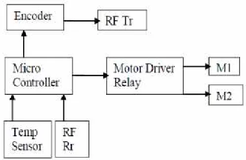
Figure 4. PC and wireless control unit block diagram

Figure 5. Sensing and Control Unit-Block Diagram

Embedded systems are integral part of our life and play a major role in improving the standard and quality of life. Consumer appliances to Bio-Medical equipment, communications, nuclear application and space research are some of the key areas where embedded systems play a vital role.

The use of micro controller has been enhanced to such an extent that we cannot expect the world without micro controller, the advantage over the much used micro processor is that it has got the internal memory to store the program which makes it more usable in the real time world. With the help of sensor feedback mechanism with RF communication the mobile robot can be controlled from a far distance, which is desirable fact when the robot is working in hazardous environment.

A potential future research avenue to extend this paper is to append the algorithm with a real-time path-planning module to which the RFID tag locations in the 3-D space would be a priori known (but not to the navigation module, however).It would also be important to

extend the capabilities of the proposed navigation system to be able to track curvilinear and circular paths.

2.

The global navigation problem deals with navigation on a larger scale in which the robot cannot observe the goal state from its initial position. A number of solutions have been proposed in the literature to address this problem. Most rely either on navigating using a pre-specified map or constructing a map on the fly. Most approaches also rely on some technique of localization. Some work on robot navigation is landmark based relying on topological maps [2], which have a compact representation of the environment and do not depend on geometric accuracy. The downside of such approaches is that they suffer from sensors being noisy and the problem of sensor antialiasing (i.e. distinguishing between similar landmarks). Metric approaches to localization based on Kalman filtering [3] Provide precision, however the representation itself is unimodal and hence cannot recover from a lost situation (Misidentified features or states). Approaches developed in recent years based on ’Markov localization’ [4] provide both accuracy and multimodality to represent probabilistic distributions of different kinds, but require significant processing power for update and hence are impractical for large environments. One of the attempts to solve this problem is presented in [5] where a sampling-based technique is used. Rather than storing and updating a complex probability distribution, a number of samples are drawn from it. The other approaches utilize partially observable Markov decision process (POMDP) models to approximate distance information given a topological map, sensor and actuator characteristics [6]. POMDP models for robotic navigation provide reliable performance, but fail in certain environments (e.g symmetric) or suffer from large state spaces (i.e. state explosion). These approaches have different advantages, but also disadvantages or fail cases. Note that all of the above approaches assume that a map of the environment (topological and/or metric) is given a priori. None of the above approaches deal with highly dynamic environments in which topology might change. Our approach, presented here, instruments the environment with a sensor network. An ant-like trail laying algorithm is presented in [7], where ‘virtual’ trails are formed by a group of robots. Navigation is accomplished through trail following. The shortcoming of the algorithm is that it is dependent on perfect communication between the members of thegroup. In addition, the ’virtual’trails are shared between the robots, which means redundant sharing of the state space in the group. Moreover, a common localization space is assumed. We are broadly interested in the mutually beneficial collaboration between mobile robots and a static sensor network.

robot navigation. Some properties of the approach are summarized below:

1) The sensor network is redeployed into the environment using the algorithm given in [8].

2) In addition to deploying the network nodes, the deployment algorithm also computes the distributions of transition probabilities P (s0js; a) from network nodes to s0, when the robot executes action a [9].

3) The nodes of the sensor network are synchronized in time (high precision is not required). For an example of a time synchronization algorithm see [10].

4) The robot does not have a pre-decided environment map or access to GPS, IMU or a compass.

5) The environment is not required to be static. 6) The robot does not perform localization or mapping.

7) The robot does not have to be sophisticated – the primary computation is performed distributive in the Sensor network, the only sensor required is for obstacle avoidance.

4.1 Probabilistic navigation

Stage I - Planning

When the navigation goal is specified (either the robot requests to be guided to a certain place, or a sensor node requires the robot’s assistance), the node that is closest to the goal triggers the navigation field computation. During this computation every node probabilistically determines the optimal direction in which the robot should move, when in its vicinity. The computed optimal directions of all nodes in conjunction compose the navigation field. The Navigation Fieldprovides the robot with the ‘best possible’ direction that has to be taken in order to reach the goal. Note that a‘kidnapped’ robot problem is solved by our system implicitly and does not require re-computation (or re-planning). It may be noted that a parallel approach for the construction of a navigation field has been proposed in the sensor network literature [11]. Instead of value iteration [11] uses potential fields and the hop count to compute the magnitude of the directional vectors.

1) Theoretical Framework - Value Iteration: Consider the deployed sensor network as a graph, where the sensor nodes are vertices. Assume a finite set of vertices S in the deployed network graph and a finite set of actions A the robot can take at each node. Given a subset of actions A(s) _ A, for every two vertices s; s0 2 S in the deployed network graph, and action a 2 A(s) the transition probabilities P(s0js; a) (probability of arriving at vertex s0 given that the robot started at

every state and then pick the actions that yield a path towards the goal with maximum expected utility.

The rationale is that the robot should ’pay’ for taking an action (otherwise any path that the robot might take would have the same utility), however, the cost should not be to big (otherwise the robot might prefer to stay at the same state). Initially the utility of the goal state is set to 1 and of the other states to 0.

2) Distributed Computation and In-network Processing:

A much more attractive solution is to compute the action policy distributive in the deployed network. The idea is that every node in the network updates its utility and computes the optimal navigation action (for a robot in its vicinity) on its

Figure 6. An example of a discrete probability distribution of vertex (sensornode) k for direction (action) “East” (i.e. right).

technique allows the robot to navigate through the environment between any two nodes of the deployed network. Note that the action policy computation is done only once and does not need to be recomputed unless the goal changes. Also, note that the utility update equations have to be executed until the desired accuracy is achieved. For practical reasons the accuracy in our algorithm is set to 10�3, which requires a reasonable number of executions of the utility update equation per state and thus, the list of utilities that every node needs to store is small. Since the computation and memory requirements are small it is possible to implement this approach on the real node device that we are using (the Mote [15]).

Note that if neighbors of all nodes are known exactly (for every direction each node has at most one neighbor), then

P (s0js; a) = 1. Hence, equations 1 and 2 reduce to the maximization of utilities of neighboring nodes only. In this case the system converges after a single iteration.

Figure 7. Navigation - node-wise approach

B. Stage II - Navigation

Note that the deployed sensor network discretizes the environment. Consider Figure 7. On the way from starting node 1 to goal node 5, the robot would first navigate from node 1 to 2, then from 2 to 3, and so on. Hence, the navigation is node wise. A node whose directional suggestion the robot follows at the moment is called current node. Initially the current node is set to the node closest to the robot. The bottom part of Figure 7 shows the three phases of navigation. Suppose initially current node is set to node 1(robot’s position at the bottom right corner on the Figure 2). Node 1 suggests the robot to go ’UP’.

In the first phase the robot accepts this command and positions itself in the correct direction. During the second phase, the robot moves ’forward’ using the VFH [2] algorithm for local navigation and obstacle avoidance. Note that throughout the second phase the current node is set to node 1. Phase 3 is triggered when the robot determines that it has entered the neighborhood of the next node -say, node 2 (an oval M2 on Figure 7). During phase 3 the current

node switches and the navigation algorithm starts from phase 1 again, but with the current node set to 2. But how to determine when the robot is in the neighborhood of some node? A straightforward approach is to use signal strength thresholding. In this case, prior to the experiment an observation model can be built which given a signal strength value would approximate the distance from the node. Hence, ideally, while in phase 2, the robot would simply collect signal strength values from the packets of all nodes in the vicinity, feed the model with these values and threshold an output picking the shortest distance.

We conducted experiments at Intel Research facilities in Hillsboro, Oregon. We used a Pioneer 2DX mobile robot, with 180o laser range finder used for obstacle avoidance, and a base station (Mica 2 mote) for communicating with the sensor network. Mica 2 motes were used as nodes of the sensor network. The sensor network of 9 nodes was redeployed into the environment. Every node is preprogrammed with information about its neighbors. We assume that the sensor network is deployed and transition probabilities set as

shortest path, and the robot should stop within 3 meters of the goal node. The algorithm allows the robot to navigate precisely and reliably using a deployed sensor network. Our approach differs from systems described in the literature by assuming that a map, localization, GPS, IMU or compass is not available. The navigation occurs through node-wise motion from node to node on the path from starting node to the goal node. We conducted 50 experiments for 5 different goals, totaling over 1 km of traveled distance. In each of the 50 cases the robot successfully navigated to the goal node. Note that we considered an experiment to be successful if the robot approached the goal node to within 3m. This distance was experimentally set as ‘good enough’. since goal nodes represent a ‘local neighborhood’ requiring robot’s presence. Hence, when the robot arrives at such a ‘localneighborhood’, local navigation algorithms, like VFH [2], can be used to drive the robot exactly to where the robot’s presence is required. Furthermore, in practice, sensor network nodes would be mounted on top of the cubicles (in places where current markers are), which makes the 3m range reasonable.

References

[1] Zadeh, L.A. Fuzzy SetsInformation and Control. 8, 1965, 338-353. Tanaka, K, An introduction to fuzzy logic for practical application, 1991.

[2] D. Kortenkamp and T.Weymouth, “Topological mapping for obile robots using a combination of sonar and vision sensing,” in Proceedings of the AAAI, 1994, pp. 979–984.

[3] K. Arras, N. Tomaris, B. Jensen, and R. Siegwart, “Multisensor on-thefly localization: Precision and reliability for applications,” Robotics and Autonomous Systems, vol. 34, no. (2-3), pp. 131–143, 2001.

[4] D. Fox, “Markov localization: A probabilistic framework for mobile robot localization and naviagation,” Ph.D. dissertation, Institute of Computer Science III, University of Bonn, 1998.

[5] F. Dellaert, D. Fox, W. Burgard, and S. Thrun, “Monte carlo localizationfor mobile robots,” inProc. of ICRA-99, 1999, pp. 1322– 1328.

[6] R. Simmons and S. Koenig, “Probabilistic robot navigation in partially observable environments,” in Proceedings of the International Joint Conference on Artificial Intelligence, 1995, pp. 1080–1087.

[7] R. Vaughan, K. Stoy, G. S. Sukhatme, and M. Mataric, “Lost: Localization-space trails for robot teams,” IEEE Transactions on Robotics and Automation, vol. 18, no. 5, pp. 796–812, 2002.

[8] M. A. Batalin and G. S. Sukhatme, “Efficient exploration without

[11] Q. Li, M. DeRosa, and D. Rus, “Distributed algorithms for guiding navigation across a sensor network,” Dartmouth, Computer Science Technical Report, Tech. Rep. TR2002-435, October 2002. [12] D. J. White, Markov Decision Process. West Sussex, England: John Wiley & Sons, 1993.