24-Hours Load Forecasting Using a Hybrid of Genetic Algorithm (GA) and Particle Swarm Optimization (PSO) for Optimized Neural Network

(1)

International Journal of Emerging Technology and Advanced Engineering

Website: www.ijetae.com (ISSN 2250-2459, ISO 9001:2008 Certified Journal, Volume 6, Issue 12, December 2016)

143

24-Hours Load Forecasting Using a Hybrid of Genetic

Algorithm (GA) and Particle Swarm Optimization (PSO) for

Optimized Neural Network

Stephen Taban Inyasio Siri Ogugu

1

, Nicodemus Abungu Odero

2

, Cyrus Wekesa Wabuge

3

1,2,3_{University of Nairobi, Department of Electrical and Information Communication, P. O. Box 30197-00100 Nairobi}

Abstract— Short-term load forecasting (STLF) has emerged as one of the most important fields of study for efficient and reliable operation of power system. It plays a very significant role in the field of load flow analysis, contingency analysis, planning, scheduling and maintenance of power systems facilities, therefore, the system n cost-effective is determine by accurate load forecast. Numerous researches have been done to improve accuracy of the conventional methods such as time series, regression analysis or ARMA and the use of artificial neural networks in load forecasting, ANN has shown lucrative results. But their training, with back-propagation algorithm or gradient algorithms is encounter long processing time, difficulty in selecting the optimal order of the components and trapping in local minima.

These researches aimed at solving this problem by proposing a hybrid based on GA and PSO for train ANN and optimize the weights of ANN. The proposed method utilized the merit of GA ability for exploration of solution in space and PSO is widely well-known by social interchanges thinking ability. This help in reducing the search space for the algorithm thus reducing the iteration time. The proposed algorithm was tested using 24 hourly load data of different days i.e. Weekdays and weekends, the results obtained were compared to those results obtained by other researchers. It was observed that HGAPSO-ANN method has a better performance in terms of reducing and improving forecast error compared to Heuristic, PSO-ANN and GA-ANN methods. It was investigated that the method the lowest APE results is HGAPSO-ANN with an approximate minimum average error is 2.734% maximum average error 6.805%, therefore, a hybridized HGAPSO algorithm with ANN to help in reducing and improving forecast error. The suggested method was programmed under MATLAB 2016® software.

Keywords—24-Hours Load Forecasting, Genetic Algorithm, Particles Swarm Optimization, HGAPSO, Artificial Neural Networks.

I. INTRODUCTION

Load forecasting is estimation of active load ahead of actual load occurrence; it is a tool that has been utilized by electricity utility such as generation, distribution, and operators as a measure for resources planning for economic dispatch[1, 2].

The purpose of load forecasting is to meet future demand, reduce unforeseen cost and provide a possible input to the decision such as systems reliability, efficiency, distribution, transmission (T&D) and the cost [3, 4, 6]. In order to plan for an efficient operation and control of power systems, the electricity utility company must able to anticipate the consumers future demand, how to deliver it, where and when [6] , thus required accurate Load forecast. Planning and controlling of load require a certain "lead time" called forecasting interval [7], depending on driving factors affecting load, this including Short-Term Load Forecasting (STLF), Mid-Term Load Forecasting (MTLF) and Long-Term Load Forecasting (LTLF)[7] [3].

As cited above, load forecasting methods classify into STLF, MTLF and LTLF methods. The STLF methods are used for hour-by-hour predictions while LTLF may be used for the peak seasonal predictions. Shown on figure 1[7]

Short-load forecasting plays a great role in power system planning, operation, and control. It enhances the energy efficiency and reliable operation of power system and helps the electric utility companies to make decisions such as unit commitment, in terms of which units are to be available, when, where to allocate them, such that it met the demand and acceptable reserve capacity, as well as the schedule plans for maintenance which unit is to be taken offline for maintenance and which unit to be dispatch into line.

II.PREVIOUS APPROACHES IN STLF

(2)

International Journal of Emerging Technology and Advanced Engineering

144

Since the load is dynamic, a deviation between historical load data and present conditions will result to large forecasting errors [12]. Fuzzy Logic[13], I. Harrison, et al

[14] conducted a study on one hour a head load used Adaptive NeuroFuzzy Interface System (ANFIS). With the development of Computational Intelligence techniques, the integrated approaches were introduced as Hybrid methods to enforce a load forecasting techniques [6] [15] [8], which are dynamically adaptable and forecasting errors is less as compared with statistical forecasting techniques. The artificial neural network ANNs has gained widely applications in various fields such load forecasting [16]fault diagnosis [17], construction cost estimations [18]. At present, some approaches have been presented to predict load using ANNs with Back Propagation (BP) algorithm [19] [20] [21], Genetic Algorithm (GA) [22], Simulating Annealing (SA) [23] Particle Swarm Optimization (PSO) [24] [25]

III. ARTIFICIAL NEURAL NETWORKS STRUCTURE

[image:2.612.61.278.448.546.2]

The common structure of Artificial Neural Network (ANN) with three layers is shown in Figure1. First layer is called the input layer, second is a hidden layer and third is an output layer for these Artificial Neural Network .The neurons of the input and hidden layers are linked by so-called synaptic weights.

Figure 1: Milt Layer Neural Network[17]

From the above Figure 1, the optimal linear combination for the ANN inputs from X1, X2, ---, Xm to neuron

hidden layers is formulated as linear summation of

m

i

x

w

h

m i i i

h

(

)

,

1 ,

2 ...

...

1







(1)

Then from hidden layers passes through an activation function to the output Yo, can be formulated as flows

m

i

x

w

f

y

m i i

i

)

,

1 ,

2 ...

...

(

1

0







(2)

Where the vector W= (w1, w2 …wn) Rn is called the

weight vector. The weights (wi)ni=1 assign to each input

synapse. It may be positive or negative. The function is called the activation function or transfer function. For this transfer function, several possible choices can be made. Assuming the transfer function is tangent sigmoid in the hidden neuron and linear activation function at output. Then, the function is given:

m j H f j H

j , 1,2...

] exp 1 [ 1 ) ( ₍ ₎    _

(3)



   n i j i ij

i w x

H

1

*



(4)

Where m is the number of inputs,

w

_ij is the weight link inputs ith to the jth hidden layers,



_j and is the threshold hidden layer, the output signal Yk is given by the

equation (5)









n j j kj

k

w

f

H

y

1

0 …

…

2 1,

=

k

,

)

(

*



(5)

Where , is weights link vector between the jth hidden layers and kth outputs layers.

For given input x the resultant learning error and mean absolute percentage error are defining the performance of the system as the total error function as follows



  m k i k y m E Error MSE 1 * ) (

(6)

100 * ) ( 1 1



   m i i i i y d y m MAPE

(7)

Where,









o i i i

k

y

d

E

1

2

)

(

, and in the number of train set, yi is the actual load and diis the demand.

A. Artificial Neural Networks learning

(3)

International Journal of Emerging Technology and Advanced Engineering

145

But there some possible disadvantage encounter by these ES, in PSO is premature convergence due to lack of momentum, which makes it not to arrive at the global optimum. By incorporating of the genetic operators into PSO, the balance between the global search of GA and social thinking ability in PSO will improve the ability of hybrid algorithm.

IV. GENETIC ALGORITHM AND OPERATORS

Genetic Algorithms (GA) is heuristic search methods inspired by natural selection (Fraser, 1957; Bremermann, 1958; Holland, 1975) [26] [27], Based on the principle of survival of the fittest,[27] It is the computational intelligent method which simulates the process of organic evolution using GA operators such as selection, crossover, and mutation[28]. Crossover point is copied from the second parent and the rest is copied from the first parent [29]. The results of the crossovers are the children. In mutation, GA randomly changes some of the genes values of the parents [30]. The salient feather of GA compare to other EA is that it search for solutions in large spaces whereby the probability of global increasing as well as the convergence[31], GA works in parallel in population not a point search, It works based on probability not deterministic[22] . In general a genetic algorithm is designed to optimize the fitness of function in search of quality of single solution in population. The fitness function depends upon system requirement. The fitness function is taken as an objective function

f

(

x

)

, Where;

n

x



₁

,

₂

,...,

, is the n-vector of optimization parameters.

The genetic algorithm GA creates a new population (called children) by applying the operators to the chromosomes in the old population (called parents). The process continues iteratively, in each iteration a new generation is created.

1) The evolution processes are as flows:

1.Initialization of the population (search space) randomly

2.Evaluation or Measure of fitness of individuals. 3.Selection of fittest individual.

4.Reproduction or application of crossover and mutation operators.

5.Replication of the above steps until convergence

V. PARTICLE SWARM OPTIMIZATION

Particles Swarm Optimization (PSO) is algorithm based on evolution theory developed which by Eberhard and Kennedy [32]. It is an optimization method based on a population of particle swarm intelligence produced by a group of particles and the competition amongst particles in a swarm[32]. In the Particles Swarm Optimization (PSO) a particle is considered as a moving point in search space with its‘ velocity and position[33]. At a time of convergence, every particle is moved toward the particles with the previous best position and the global best position. A new velocity acquired by each particle is calculated in an iteration based on its current velocity and the location from its previous best position and the global best position[33]. The PSO process involves the updating of a particle velocity and position with time until the best solution is obtained.

2) PSO implementation Steps: The particle swarm optimization algorithm, the swarm has population particles represent set of m possible solution, where m is the vector number of optimized parameters. Therefore, each m parameter represents a dimension of the problem in space.

The Particle Swarm Optimization Algorithm sequential steps,

1.Initialization: Allocate the initial parameters, such as velocity, inertia weight, acceleration constants, and randomly generates initial population of n particles. 2.Calculate the Fitness: For all n particles, evaluate the

fitness value for each particle according to Equation (6). 3.Compare the fitness value of each particle (16) using

objective function and save as pbest for each particle, and determining the gbest as the best value obtained. 4.Movement and location: Updating the velocity and

location of each particle based on Equations (13) and (14)

5.Updating the gbest and pbest: Evaluating the fitness values of the particles and updating gbest and pbest values using Equations (16)

6.Stop criteria: If the stoppage criteria are satisfied, go to step 7, otherwise proceed to step 2

7.Stop the simulation

(4)

International Journal of Emerging Technology and Advanced Engineering

146

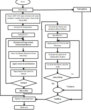
VI. PROPOSED METHODOLOGY

There are several ways of combining these two optimization techniques to come out with a better approach to solve difficult problem at hand, such optimization problems, adjusting the weight and bias of the neural network. In this research work, a hybrid metheuristic algorithm proposed for training ANN by combining GA with PSO. The concept behind this hybrid is to combine the search abilities of genetic algorithm GA and particle swarm optimization PSO for optimizing the weights of ANN. This combination provides global exploration of the search space and the local exploitation of different discovered regions in the search space

The proposed hybrid method works as follows. First, initialization of population n-pop of n candidate solutions is

generated randomly within the interval [xMax, xMin], for each iteration

(

It

)

of algorithm. Using GA selection and recombination operations are applied in n-pop to produce new solutions in current population. The current population

n-popt-1 is enhanced and evaluated according to the

(5)

International Journal of Emerging Technology and Advanced Engineering

[image:5.612.129.492.146.586.2]

147

(6)

International Journal of Emerging Technology and Advanced Engineering

148

VII. ANN REPRESENTATION AS ACHROMOSOME

The total number of weights of ANN depends on the number of neurons in input, hidden and output layer which is calculated by

]

)

*

(

)

*

(

[

T.N.Ws



In

_n

H

_n



H

_n

O

_n



H

_n



O

_n

(8)

Where

n

In is number of input neurons,

n

H is number of hidden neurons which correspond to the bias weights and

O

_nis number of output neurons. The initial weights are randomly initialized within the interval [xMax, xMin], and each weight represent the weighted link between the neurons of the layers to another. Since a chromosome contains group of genes, a set of weights in ANN can be represented by number of N-gene, where every gene corresponds to each weighted link in the network. Therefore, each chromosome represents ANN and the gene of the chromosome represents the weights of Artificial Neural Network. The fundamental elements of a genetic algorithm GA that should be specified for any given implementation are representation, number of population, evaluation, selection, operators and parameters. These elements are described below:

B. Population Initialization

The n-chromosomes A is initialized randomly as vectors

n-genes within the interval [xMax, xMin] each of these vectors is a possible solution in search space of the problem.

C. Roulette Wheel Selection Method

In the roulette wheel approach, a probability of selection

i

p

assigns to each individual q according to its fitness value. Each individual is sort based on their fitness which reflects the fitness of the previous individual chromosome. So a series of n-random numbers is generated and contrasted to the cumulative probability





 n

q i

i p

cp

1

of the population.Huang et al [34] State that if the fitness of individual i in the population is fi(x), its chance of being

selected to next generation is





 _n

1 q

q i i

(x) f

p

(9)

Where n is the number of individual in the population, and

f(x)

is the fitness of individual i. Thus, each individual has a chance to become a parent in next generation based on its fitness in the population. In other selection methods, the individuals with better fitness have highest chances of selection which is biased. It‘s can also perhaps neglect the best individuals of a population, there is no assurance that all best individuals will pass to next generation. The virtual roulette wheel is spanned, the individual corresponding to the section on which roulette wheel stops are then selected, hence each individual with best or worst fitness has chances of being pass to next generation. This is a merit, however the solution may be having weak results, but it could be useful for following regeneration process. In this research work, the algorithm employed GA to do exploration while roulette wheel selection technique was used to creation selection, thus making the process the most complimentary.

D. Crossover and Mutation

It could be believed that the main unique element of a GA is the use of crossover. In this research project, the arithmetic crossover, which is used for floating point representations, such as real coded recombination of

n-vectors, which represent number of children in proposed algorithm, and the mutation is to flip an individual randomly in the solution‘s space. These operators help in avoiding early convergence optimism and thus improving the performance of algorithm. In Bodenhofer et al 2004

[35] assumed that dealing with a free n-dimensional real-coded optimization problem, says

Χ



R

n. The individual is then represented as an n-dimensional vector of real numbers.

)

x

,...,

(x

a



₁ _n

E. Flat Crossover

Given two parents

a

₁



(x

1₁

,...,

x

1_n

)

and

a

₂



(x

₁2

,...,

x

_n2

)

, to reproduce the new offspring

)

x

,...,

(x

a

'



'₁ '_n (for all i=1… n). Arithmetic crossover, which is used for floating point representations, children is calculated as the arithmetic mean of the parents

childB childA

childA

β*

x

[1

β]

*

x

(7)

International Journal of Emerging Technology and Advanced Engineering

149

childA

childB

β*

x

[1

β]

*

x

X







(10b)

Where

β

_ia uniformly distributed random value from the unit interval is used to compute the offspring,

F. Mutation

Mutation is used to explore new areas in the search space and to add diversity to the population of chromosomes in order to avoid being trapped in a local optimum. The crossover operator proposed for the real coded GA to randomly selected gene i of a chromosomes

a



(x

₁

,...,

x

_n

)

the allele

x

_i is randomly selected value from a predefined interval[ai,bi].

Mutation is applied to the children chromosomes after crossover is performed. The mutation method used is floating point no uniform mutation, where kth element of X chromosome, X mutated equation is described as follows:

k k

k

_Δx

x





(11)

)

rand

)(1

(x

Δx

k





k



(1It/MaxIt)ψ

xMin

(12a)

)

rand

)(1

(x

Δx

k





k



(1It/MaxIt)ψ

xMin

_(12b)

Where xMax and xMin are the maximum and minimum values of search space, it is the current iteration; MaxIt is maximum number of iterations and ѱ is the parameter determining the degree of iteration. In proposed GA algorithm flat crossover and mutation was employed to avoid the process of encoding and decoding of the chromosomes, thus contributed on making the algorithm less the complex and facilitated in reducing its computation time.Siriwardere et al. (2006)[36] investigated the effects of the variation and selection of crossover and mutation probabilities for urban drainage model optimization. They propose a crossover probability of 80% and a mutation probability of 1% as the best figures to work with during optimization. Therefore, 80% crossover and 1% mutation profanities have been used in this research work.

VIII.PARTICLE SWARM OPTIMIZATION ALGORITHM (PSO) The new individuals created from real-coded GA are passed to PSO; where PSO applied the velocity and position update of individuals called particles. The process updating the velocity and position of particles involves selection of the best particles, selection of the global best particle, and finally velocity updates.

The global best particle of the swarm is determined according to the sorted fitness values. The best particles are selected by first dividing the n particles into n

neighborhoods and assigning the particle with the better fitness in each neighborhood as the neighborhood best particle. The equations (13) and (14) demonstrate the velocity and position updates of the particle.

])

[

]

[

(

..

])

[

]

[

(

]

[

]

1 [

2 2 1 1

t

x

t

gbest

r

c

t

x

t

pbest

r

c

t

wV

t

V

i i i i i













(13)

]

1 [

]

[

]

1 [

t





X

t



V

t



X

_i _i _i

(14)

Where, Xi(t) is the position of the particle i at time

t,V_i[t]is the velocity of particle i at time

t,

pbest

_i

[

t

]

is the best position found by particle itself so far,

gbest

[

t

]

is the best position found by particle in a swarm. , and are the initial values of learning coefficients factors influencing the

pbest

_i

[

t

]

, and

]

[

t

gbest

position of the particle, and are random variables within the range of (0, 1). Thus, the following linear formulation of inertia weight ω and learning factors which provides a balance between global and local search are utilized as follows:

It

_max

*

min max max







(15)

max

min







Where ω is an inertia weight scaling the previous time step velocity,



_max and



_min represent the maximum and minimum values of inertia weight.

It

, is the current number of iterations and

It

_max is the maximum number of allowable iterations.

Equations (16) define how personal and global best are updated at time [t]. Objective function f is to calculate the fitness of the particles with a minimization task.

Thus, i (1…s) if

] 1 [ ] 1 [ ] 1 [ ( ] [ ( ] [ ]) 1 [ ]) 1 [ ( ]) [ (            t x t pbest t x f t pbest f t pbest t pbest t x f t pbest f i i i i i

(16)

])}

[

(

),

(

min{

]

(8)

International Journal of Emerging Technology and Advanced Engineering

150

Where, ]} [ ..., ],... [ ], [

{pbest₀ t pbest₁ t pbest₂ t y

IX. PREDICTION AND DATA PROCESSING

Modeling with ANNs, requires an appropriate selection and preparation of input data to minimize the variation of sampled input data and the output data to improve the accuracy, first, the original data set needs to be normalized. In this works the linear transformation technique is used to normalize the data, shown as follows:

n) … 2 (1, = i , minX maxX minX X X i n _  

(17)

Where Xi is the sampled data, maxX and minX are the

maximum and minimum values of the sampled data, and the Xn is the sampled data matrix vector converted within

[0, 1] after the normalization process. X.CORRELATION ANALYSIS

DeCoursey at el. 2003 [37] correlation analysis is determine the relationship between two variables, say X

and Y both variables are assumed to be varying randomly. Peter X-K, Song atel. 2007 [38] assume for the analysis that the variables X and Y are related linearly, the correlation coefficient gives a measure of the linear relationship between X and Y, can be calculated as follows;









n 1 i 2 i

xx

(x

x

)

S

(18)









n 1 i 2 i

)

(

S

_yy

y

(19)









n 1 i 2 i 2

i

)

(

)

(

S

_xy

x

y

(20)

yy xx xy xy

S

r



(21)

Where, Sxx is sum of squares for x, Syy is sum of squares for y and Sxy is sum of products for x and y and rxy

is correlation coefficient.

TABLE I

ILLUSTRATIONS OF VARIOUS CORRELATION COEFFICIENTS

Correlation (X, Y)

rxy =+1 Positive correlation

rxy =-1 Negative correlation

rxy =1 Perfect correlation

rxy =0 No systematic relation between X and Y

0< rxy<0.09 Represents no correlation

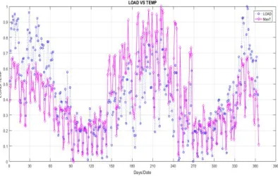
The samples, historical load data and weather data for analysis were obtained of Juba Power Station (JPS) and Juba International Air Weather Station (JIAWS) for the year 2010 were used to obtained information about the relationship between the load and weather variables. The regression analysis presumes that the independent variable has no error, but there is random error in the dependent variable.

TABLE II

CORRELATION ANALYSIS RESULTS

Variable correlation coefficient Relative Humidity, Load 0.3265

Temperature, Load 0.6917

[image:8.612.323.565.156.237.2]

From the Table II of correlation analysis above, which show the correlation between load and weather variables, the analysis shows the temperature has significant effect on the load contrast to relative humidity, hence, temperature will be include in load forecasting.

Figure 3: One year load and temperature

[image:8.612.51.218.478.616.2] [image:8.612.343.540.484.612.2]

(9)

International Journal of Emerging Technology and Advanced Engineering

[image:9.612.200.411.143.278.2]

151

Figure 4: Daily load curves for one week, Monday, Tuesday, Wednesday, Thursday, Friday, Saturday & Sunday

TABLE III

SIMULATION PARAMETERS FOR GA AND PSO

Parameter PSO GA Description

Number of particles n 50 50 Population Size (Swarm Size) Maximum Iteration 100 100

Cognitive coefficient c1 1.5 - Personal Learning Coefficient Social coefficient c2 2.5 - Global Learning Coefficient

Inertial weight ω 0.1+rand*0.4 - Determine the influence of the current velocity Max. weight 0.9 -

Min. weight 0.4 -

Vmax +5 - Max. velocity Vmin -5 - Min. velocity

xMax 1 - Upper bound of swarm xMin 0 - Lower bound of swarm Beta - 8 Selection Pressure Pc - 0.8 Crossover Percentage Pm - 0.01 Mutation Percentage Mu - 0.1 Mutation Rate

XI. INPUT AND OUTPUT FOR THE HYBRID HPSO MODEL

The data obtained of Juba Power Station (JPS) and Juba International Air Weather Station (JIAWS) for the year 2010, were clustered as weekdays from Monday through Friday, Saturday and Sunday as weekend due to the different load profile of working day and weekend, the weekdays load curves have relatively similar shape for different weeks. Figure 4 Show daily load curves for one week, Monday, Tuesday, Wednesday, Thursday, Friday, Saturday & Sunday. The inputs to hybrid model used 24-hour load of same day, of previous day, 168-24-hour load of same day previous week. One layer for output representing time a head 24-hour load forecast for next day.

The idea behind clustering the data and taking specific inputs, is to takes a consideration of 24-hour of the day effect to map 24-hourly load variation and days of the Week is taken into account to reflect the weekly load pattern on weekdays and weekends.

XII. SIMULATION PROCESS

The simulation process for getting the forecast results, which is the network learning process, can be summarized below:

[image:9.612.85.530.324.537.2]

(10)

International Journal of Emerging Technology and Advanced Engineering

152

2.The data is loaded to Mat lab workspace from an excel file ‗datafile.xlsx‘.

3.The ‗datafile.xlsx‘ file is read using ‗xlsread‘ function load inputs and target.

4.The network is then created ‗fit net‘, with number of inputs and output. The number of hidden layer is selected based on trial and error since there in not rule for determining the number of hidden layers of neural network.

5.The network is trained using historical data. In this study, the data used for the training is from May-July 2010.

6.After the training process is finished, the network is validated using the data from July 2010.

7.The output of the network is renormalized to get a contrast the actual data and the output results of the model which are written down.

8.The performance of the network is the evaluated by using mean absolute performance error (MAPE) and absolute performance error APE.

In this research, a HGAPSO is used to train the ANN network by alternating the weights such that the resulting mean square error (MSE) for the training data is minimized. The training process runs until the maximum number of iterations has been reached (see Table IV, Table V and Table VI).The values in the Table IIIwere adopted by Mishra at el 2008 [39] and validated by experimentation with other values.

The chromosome in GA corresponds to particles in swarm and the particle position in the search space of the PSO corresponds to the weights of the ANN. The fitness function f is mean square error (MSE) of the ANN. Each particle represents a possible solution of weights. The number of hidden layer neurons in each ANN was set at 5 to 100. These values were selected by trial and error to determine the minimum number of hidden-layer neurons that would produce the lowest forecast error and the network topology was taken based on the results.

(11)

International Journal of Emerging Technology and Advanced Engineering

153

TABLE IV

PERFORMANCE EVALUATION OF HGAPSO-ANNMODEL

Day Network Inputs

Hidden

neuron APE MAPE R

Day Network APE MAPE R APE

W

ee

k

d

ay

HGAPSO

-A

NN

24

5 1.419 0.059 0.992

W

ee

k

d

ay

PSO

-ANN

(12)

International Journal of Emerging Technology and Advanced Engineering

154

TABLE V

Performance Evaluation of GA-ANN Model

Day Network Inputs Hidden neuron APE MAPE R

W

ee

k

d

ay

GA

-ANN

24

5 20.050 0.201 0.986 10 17.809 0.742 0.996 15 7.891 0.329 0.989 20 11.759 0.490 0.971 25 5.721 0.238 0.999 30 2.201 0.092 0.995 35 3.620 0.151 0.986 40 8.917 0.372 0.968 45 5.939 0.248 0.999 50 14.816 0.617 0.964 55 16.991 0.708 0.970 60 12.540 0.523 0.989 65 3.497 0.146 0.991 70 12.402 0.517 0.966 75 3.019 0.126 0.991 80 4.831 0.201 0.995 85 7.978 0.332 0.995 90 20.050 0.835 0.964 95 6.171 0.257 0.607 100 1.271 0.053 0.962 XIII.RESULTS AND DISCUSSION

This section presents the results of different 24-hour load forecasts using trained ANNs. The MAPE and APE for the forecaster inputs are presented to shows the significant of the approaches and graph plots for the predictor inputs are also been presented to visually see the correlations and trends between the forecasters and the actual load. To reduce the size and complexity of the forecaster analysis, the correlation analysis results for chosen 24-hour load forecast days are tabularized and discussed.

Load forecast results are presented along with 24-hour load forecast profile plots for selected days.

(13)

International Journal of Emerging Technology and Advanced Engineering

155

TABLE VI

MAPE(25-31/07/2010) AND APE(25-31/07/2010)

MAPE for Different days APE for Different days

Day

PSO-ANN GA-ANN

HGAPSO-ANN Day

PSO-ANN

GA-ANN

HGAPSO-ANN

Working Day

0.0135 0.0241 0.1388

Working Day

0.325 0.579 3.331 0.1603 0.1636 0.0106 3.848 3.926 0.255 0.1826 0.1667 0.0349 4.383 4.001 0.838 0.1229 0.0929 0.0076 2.951 2.229 0.184 0.0803 0.058 0.0616 1.928 1.392 1.479

Weekend

0.0198 0.0886 0.0891

Weekend

0.476 2.127 2.137 0.0355 0.1939 0.0019 0.853 4.654 0.046 Average 0.0880 0.113 0.049 Average 2.109 2.701 1.181

TABLE VII

CORRELATION R(04-10/11/2010) AND CORRELATION R(06-13/11/2010)

Daily Load R 2010 Networks Daily Load R 2010 Network

Day

PSO-ANN GA-ANN

HGAPSO-ANN Day

PSO-ANN

GA-ANN

HGAPSO-ANN

Working Day

0.992 0.964 0.975

Working Day

0.963 0.957 0.961 0.995 0.974 0.983 0.969 0.957 0.964 0.994 0.993 0.994 0.982 0.977 0.982 0.997 0.995 0.997 0.964 0.952 0.959 0.982 0.985 0.987 0.979 0.972 0.977

Weekend

0.949 0.962 0.964

Weekend

0.968 0.991 0.990 0.990 0.993 0.993 0.964 0.989 0.987

TABLE VIII

ONE WEEK FORECAST MODELS COMPARISON

Week Forecast

NETWORK MAPE APE R PSO-ANN 0.002 0.276 0.992 GA-ANN 0.010 1.691 0.990 HGAPSO-ANN 0.000 0.009 0.987

G. Load Forecast Results

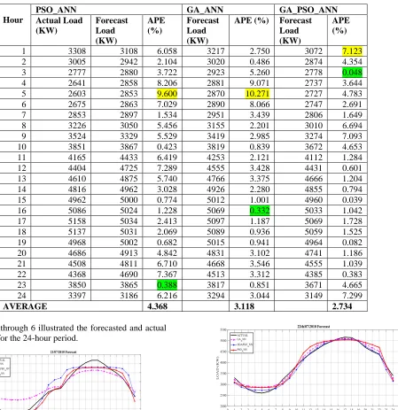
The 24-hour-ahead load forecast results for selected days from a week are tabularized in Table IX. The APE results for forecasters (PSO-ANN, GA-ANN and HGAPSO-ANN) have an approximate average range of 4.37% to 5.61 %, 3.113% to 6.25%, and 2.73% to 4.81% respectively. These errors are comparable to the APE results found in the STLF literature [40][41][42][43].

(14)

International Journal of Emerging Technology and Advanced Engineering

156

TABLE IX

24-HOULY FORECAST RESULTS DATE 22/07/2010

Figures 5 through 6 illustrated the forecasted and actual load shapes for the 24-hour period.

[image:14.612.100.549.154.617.2]

Figure 5: 24-Actual and forecasted load profile for 21th July 2010

Figure 6: 24-Actual and forecasted load profile for 22th July 2010

Hour

PSO_ANN GA_ANN GA_PSO_ANN

Actual Load (KW)

Forecast Load (KW)

APE (%)

Forecast Load (KW)

APE (%) Forecast Load (KW)

APE (%)

1 3308 3108 6.058 3217 2.750 3072 7.123 2 3005 2942 2.104 3020 0.486 2874 4.354 3 2777 2880 3.722 2923 5.260 2778 0.048 4 2641 2858 8.206 2881 9.071 2737 3.644 5 2603 2853 9.600 2870 10.271 2727 4.783 6 2675 2863 7.029 2890 8.066 2747 2.691 7 2853 2897 1.534 2951 3.439 2806 1.649 8 3226 3050 5.456 3155 2.201 3010 6.694 9 3524 3329 5.529 3419 2.985 3274 7.093 10 3851 3867 0.423 3819 0.839 3672 4.653 11 4165 4433 6.419 4253 2.121 4112 1.284 12 4404 4725 7.289 4555 3.428 4431 0.601 13 4610 4875 5.740 4766 3.375 4666 1.204 14 4816 4962 3.028 4926 2.280 4855 0.794 15 4962 5000 0.774 5012 1.001 4960 0.039 16 5086 5024 1.228 5069 0.332 5033 1.042 17 5158 5034 2.413 5097 1.187 5069 1.728 18 5137 5031 2.069 5089 0.936 5059 1.525 19 4968 5002 0.682 5015 0.941 4964 0.082 20 4686 4913 4.842 4831 3.102 4741 1.186 21 4508 4811 6.710 4668 3.546 4555 1.039 22 4368 4690 7.367 4513 3.312 4385 0.383 23 3850 3865 0.388 3817 0.851 3671 4.665 24 3397 3186 6.216 3294 3.044 3149 7.299

[image:14.612.75.263.549.645.2]

(15)

International Journal of Emerging Technology and Advanced Engineering

157

XIV. CONCLUSION

In this study the main objective was to develop hybrid method for short term load forecasting models using Genetic Algorithm and Particle Swarm Optimization (HGAPSO-ANN) to train Artificial Neural Network. The results of HGAPSO-ANN were compared to PSO-ANN and GA-ANN in order to determine the better method with good results. The performances of these models were evaluated using the absolute percentage error (APE). It was investigated that the method with the lowest APE results is HGAPSO-ANN with an approximate minimum average error is 2.734% maximum average error 6.805%, therefore, a hybridized HGAPSO algorithm with ANN help in reducing and improving forecast error. A hybrid PSO-ANN was also investigated where particle swarm optimization was utilized to adjust the weights of the Artificial Neural Network the resulting absolute percentage error (APE) was found to be good with an approximate average range of 3.88% to 7.53 %, as well as GA-ANN was examined the resulting absolute percentage error (APE) was found to be good with an approximate average range 3.113% to 8.037%. Therefore, by introducing hybridization concept, the minimum forecast error results can be obtained.

The observation from this work is that the proposed method has better forecasting results.

REFERENCES

[1] D. K. and I. . Nagrath, Modern Power System Analysis, Third Edit. New Delhi: Tata McGraw Hill Education Private Limited, 2003. [2] H. L. Willis, Spatial Electric Load Forecasting, Second Edi. New

York.: Marcel Dekker, Inc., 2002.

[3] F. Javed, N. Arshad, F. Wallin, I. Vassileva, and E. Dahlquist, ―Forecasting for demand response in smart grids: An analysis on use of anthropologic and structural data and short term multiple loads forecasting,‖ Appl. Energy, vol. 96, pp. 150–160, 2012.

[4] E. a Feinberg and D. Genethliou, ―Load Forecasting,‖ Appl. Math. Restructured Electr. Power Syst., pp. 269–285, 2005.

[5] F. J. Nogales, J. Contreras, A. J. Conejo, and R. Espínola, ―Forecasting next-day electricity prices by time series models,‖ IEEE Trans. Power Syst., vol. 17, no. 2, pp. 342–348, 2002. [6] E. Almeshaiei and H. Soltan, ―A methodology for Electric Power

Load Forecasting,‖ Alexandria Eng. J., vol. 50, no. 2, pp. 137–144, 2011.

[7] Hossein Seifi and Mohammed Sadegh Sepasian, Electric Power System Planning, S. Springer Heidelberg Dordrecht London New Yerk, 2011.

[8] M. C. W Charytoniuk, ―Very Short term load forecasting using Artificial Neural Networks‖, IEEE Transactions on Power Systems,‖ IEEE Trans. Power Syst., vol. Vol.15,, no. No. 1, p. PP .263 – 268. [9] J. Nowicka-zagrajek and R. Weron, ―Modeling electricity loads in

California : ARMA models with hyperbolic noise,‖ Signal Procesign, vol. 82, pp. 1903–1915, 2002.

[10] J. Automation, S. L. Forecasting, U. Time, and A. Moving, ―2 . Time Series and Data Mining 3 . Forecasting Methods,‖ vol. 3, pp. 122– 132, 2014.

[11] S. A. H.M. Al-Hamadi, Soliman, ―Short-term electric load forecasting based on Kalman filtering algorithm with mo v ing window weather and load model,‖ Electr. Power Syst. Res., vol. 68, 2004.

[12] H. M. Al-Hamadi and S. a. Soliman, ―Short-term electric load forecasting based on Kalman filtering algorithm with moving window weather and load model,‖ Electr. Power Syst. Res., vol. 68, no. 1, pp. 47–59, 2004.

[13] S. a. Soliman, Fuzzy Regression Systems and Fuzzy Linear Models. 2010.

[14] I. O. Harrison, ―Short Term Electric Load Forecasting of 132 / 33KV Maiduguri Transmission Substation using Adaptive Neuro-Fuzzy Inference System ( ANFIS ),‖ Int. J. Comput. Appl., vol. 107, no. 11, pp. 23–29, 2014.

[15] P. S. R. Murty, Power System Analysis. Giriraj Lane, Sultan Bazar,: BS Publications, 2007.

[16] I. K. Ibraheem, D. Ph, and M. O. Ali, ―Short Term Electric Load Forecasting based on Artificial Neural Networks for Weekends of Baghdad Power Grid,‖ Int. J. Comput. Appl., vol. 89, no. 3, pp. 30– 37, 2014.

[17] N. I. E. Shan-kun, W. Yu-jia, X. Shanli, and C. Ke, ―A Hybrid of Particle Swarm Optimization And Genetic Algorithm for Training Back-Propagation Neural Network,‖ Int. J. Res. Eng. Sci., vol. 4, no. 5, pp. 48–58, 2016.

[18] G. Feng and L. Li, ―Application of Genetic Algorithm and Neural Network in Construction Cost Estimate,‖ in Proceedings of the 2012 2nd International Conference on Computer and Information Application (ICCIA 2012), 2012, no. Iccia, pp. 1036–1039. [19] J. López, M. Valero, S. Senabre, C. Aparicio and A. Gabaldon,

―Application of SOM neural networks to short-term load forecasting: The Spanish electricity market case study,‖ Electr. Power Syst. Res., vol. 91, pp. 18–27, 2012.

[20] A. Ghanbari et al., ―Expert Systems with Applications A new hybrid Modified Firefly Algorithm and Support Vector Regression model for accurate Short Term Load Forecasting,‖ Expert Syst. Appl., vol. 41, no. 13, pp. 541–548, 2010.

[21] G. Liao and T. Tsao, ―Application of fuzzy neural networks and artificial intelligence for load forecasting,‖ Electr. Power Syst. Res., vol. 70, pp. 237–244, 2004.

[22] B. Islam, Z. Baharudin, Q. Raza, and P. Nallagownden, ―Hybrid and Integrated Intelligent System for Load Demand Prediction,‖ in B. Islam, Z. Baharudin, Q. Raza el at., 2013, no. June, pp. 178–183. [23] S. Quaiyum, Y. I. Khan, S. Rahman, and P. Barman, ―Artificial

Neural Network based Short Term Load Forecasting of Power System,‖ Int. J. Comput. Appl., vol. 30, no. 4, pp. 1–7, 2011. [24] S. Yu, K. Wang, and Y. Wei, ―A hybrid self-adaptive Particle

Swarm Optimization – Genetic Algorithm – Radial Basis Function model for annual electricity demand prediction,‖ Energy Convers. Manag., vol. 91, pp. 176–185, 2015.

[25] Z. A. Bashir, ―Applying Wavelets to Short-Term Load Forecasting Using PSO-Based Neural Networks,‖ IEE Trans. Power Syst., vol. 24, no. 1, pp. 20–27, 2009.

[26] J. Mcilwraith and J. Stark, Decision Engineering. Springer, 2008. [27] M. G. R. Cheng, Genetic Algorithms & Engineering Optimization,

(16)

International Journal of Emerging Technology and Advanced Engineering

158

[28] Q. Zhu and A. T. Azar, Complex System Modelling and Control

Through Intelligent Soft Computations, vol. 319. 2015. [29] K. Sastry and D. Goldberg, GENETIC ALGORITHMS. 1975. [30] F. Elkarmi and N. Abu Shikhah, Power System Planning

Technologies and Applications. 2012.

[31] R. Lowen and A. Verschoren, Foundations of generic optimization Volume 2, R. Laubenb. Springer, 2008.

[32] A. Jain, M. B. Jain, and E. Srinivas, ―A Novel Hybrid Method for Short Term Load Forecasting using Fuzzy Logic and Particle Swarm Optimization,‖ in International Conference on Power System Technology, 2010, pp. 1–7.

[33] P. Duan, K. Xie, T. Guo, and X. Huang, ―Short-Term Load Forecasting for Electric Power Systems Using the PSO-SVR and FCM Clustering Techniques,‖ Energies, vol. 4, pp. 173–184, 2011. [34] M.-W. Huang et al, ―A genetic algorithm for sequencing type

problems in engineering design,‖ Int. J. Numer. Methods Eng., vol. 40, no. 17, pp. 3105–3115, 1997.

[35] U. Bodenhofer, Genetic Algorithms: Theory and Applications, Third Edit. Fuzzy Logic Laboratorium-Hagenberg, 2004.

[36] N. R. Siriwardene and B. J. C. Perera, ―Selection of genetic algorithm operators for urban drainage model parameter optimisation,‖ vol. 44, pp. 415–429, 2006.

[37] W. J. DeCoursey, Statistics and Probability for Engineering Applications. Elsevier Science (USA), 2003.

[38] Peter X.-K. Song, Springer Series in Statistics, 2nd ed. Springer Science+Business Media, LLC, 2007.

[39] S. Mishra and S. K. Patra, ―Short term load forecasting using neural network trained with genetic algorithm & particle swarm optimization,‖ Proc. - 1st Int. Conf. Emerg. Trends Eng. Technol. ICETET 2008, pp. 606–611, 2008.

[40] Y. Shangdong, ―A New ANN Optimized By Improved PSO Algorithm Combined With Chaos And Its Application In Short-term Load Forecasting,‖ 2006, pp. 945–948.

[41] N. K. Singh, A. K. Singh, and M. Tripathy, ―Short Term Load Forecasting using Genetically Optimized Radial Basis Function Neural Network,‖ in IEEE POWER ENGINEERING INTERNATIONALCONFERENCE, 2014, no. October, pp. 1–5. [42] P. N. S. H. I. Ying-ling, ―Research on Short-Term Load Forecasting

Based on Adaptive Hybrid Genetic Optimization BP Neural Network Algorithm,‖ no. 70572090, pp. 1563–1568, 2008. [43] X. Sun et al., ―An Efficient Approach to Short-Term Load