An Exact Method to Compute Time Delay Margin for Stability of Time- Delayed Generator Excitation Control System

(1)

Page 276

An Exact Method to Compute Time Delay Margin for Stability of

Time-Delayed Generator Excitation Control System

Sahin Sonmez

1

_{, Ulas Eminoglu}

2

_{Saffet Ayasun}

3

1

PhD Student, Department of Electrical and Electronics Engineering, Nigde University, Nigde, Turkey.

2

_{Associate Professor, Department of Electrical and Electronics Engineering, Nigde University, Nigde, Turkey.}

3

_{Professor, Department of Electrical and Electronics Engineering, Nigde University, Nigde, Turkey.}

---*---Abstract -**

This paper investigates the effect of time

delays on the stability of a generator excitation control system compensated with a stabilizing transformer known as rate feedback stabilizer to damp out oscillations. The time delays are due to the use of measurement devices and communication links for data transfer. A direct and exact method based on Rekasius substitution is proposed to determine the maximum amount of time delay known as delay margin that the system can tolerate without loosing its stability. The proposed method starts with the determination of all possible purely imaginary characteristic roots for any positive time delay. To achieve this, Rekasius substitution is first used to convert the transcendental characteristic equation into a polynomial. Then, Routh stability criterion is applied to determine the critical root, the corresponding oscillation frequency and the delay margin for stability. It is found that the excitation control system becomes unstable when the time delay crosses certain critical values. Theoretical delay margins are computed for a wide range of controller gains and their accuracy are verified by using Matlab/Simulink. Results also indicate that the addition of a stabilizing transformer to the excitation system increases the delay margin and improves the system damping significantly.

Key Words:

Excitation control system, Time delay,

Delay margin, Stability, Rekasius substitution.

1. INTRODUCTION

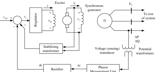
In electrical power systems, load frequency control (LFC) and excitation control system also known as automatic voltage regulator (AVR) equipment are installed for each generator to maintain the system frequency and generator output voltage magnitude within the specified limits when changes in real and reactive power demand occur [1, 2]. This paper investigates the effect of the time delay on the stability of the generator excitation control system that includes a stabilizing transformer by using an exact and direct analytical method. Figure 1 shows the schematic

block diagram of a typical excitation control system for a large synchronous generator. It consists of an exciter, a phasor measurement unit (PMU), a rectifier, a stabilizing transformer (rate feedback stabilizer) and a regulator [1]. The exciter provides DC power to the synchronous generator’s field winding constituting power stage of the excitation system. Regulator consists of a proportional-integral (PI) controller and an amplifier [2,3]. The regulator processes and amplifies input control signals to a level and form appropriate for control of the exciter. The PI controller is used to improve the dynamic response as well as to reduce or eliminate the steady-state error. The amplifier may be magnetic amplifier, rotating amplifier, or modern power electronic amplifier.

The PMU derives its input from the secondary sides of the three phases of the potential transformer (voltage transducer) and outputs the corresponding positive sequence voltage phasor. The rectifier rectifies the generator terminal voltage and filters it to a DC quantity. The stabilizing transformer provides an additional input signal to the regulator to damp power system oscillations [4].

The operation of this system can be described as follows: When an increase in the power load demand, especially in the reactive power load demand occurs, a drop in the generator terminal voltage (Va ) is observed. The voltage

magnitude is sensed by the PMU through a potential transformer. The measured voltage is rectified and compared with a reference DC voltage. The PI controller produces an analog signal that controls the firing of a controlled rectifier shown as amplifier in Figure 1. Thus, the regulator (PI controller and amplifier) controls the exciter field and increases the exciter terminal voltage.

(2)

Page 277

Rectifier

Potential transformers Stabilizing

transformer

R

eg

u

la

to

r

G

+ +

_ _

ref

v ve

R

v vf

∆P ∆Q Synchronous

generator Exciter

ac dc

To rest of system

i if Va

+

_ _

Voltage (sensing) transducer Phasor Measurement Unit

Fig -1:The schematic block diagram of the generator excitation control system

_

Amplifier Exciter Generator

Sensor and rectifier

) (s

Vref VE( )s V sR( ) VF( )s V sT( )

PI Controller

( ) I

C P

K G s K

s

 

Measurement and Communication

signal delay

( ) 1

G G

G K G s

T s 



( ) 1

E E

E K G s

T s 



( ) 1

A A

A K G s

T s 



s

e ( )

1

R R

R K G s

T s 



+

( )

S V s

( ) 1

F F

F K s G s

T s 



Stabilizer

Fig -2: Block diagram of excitation control system including time delay

In past studies [6-7], time delay was usually considered as constant value. However, in real power systems it usually fluctuates randomly in some range. Therefore, it is vital to determine the maximum amount of time delay known as delay margin that the system can tolerate without becoming unstable. There are several methods in the literature to compute delay margins of time-delayed continuous systems such as the generation excitation control system. The common starting point of them is the determination of all the imaginary roots of the characteristic equation. The existing procedures can be classified into the following five distinguishable approaches: i) Schur-Cohn (Hermite matrix formation) [8-10]; ii) Elimination of transcendental terms in the characteristic equation [11]; iii) Matrix pencil, Kronecker sum method [8-10, 12]; iv) Kronecker multiplication and elementary transformation [13]; v) Rekasius substitution [14-17]. These methods demand numerical procedures of different complexity and they may result in different precisions in computing imaginary roots. A detailed comparison of these methods, demonstrating their strengths and weakness can be found in [18].

Among these methods, we have applied the method presented in [11] into the delay margin computation of excitation control system without a stabilizing transformer [19]. This paper aims to extend our earlier work by proposing a more efficient and less complex method as compared with one given in [11] to determine

delay margin for stability of the time-delayed excitation control system.

[image:2.595.163.429.104.227.2] [image:2.595.151.449.257.371.2]

(3)

Page 278

Moreover, in this current study, the excitation control

system model studied in [19] is enhanced by including a stabilizing transformer. With this enhancement, it will be possible to investigate the impact of a stabilizing transformer to the delay margin and the stability of time-delayed generator excitation control system. Such analyses do not exist in the literature. Using the proposed method, the delay margins are computed for a wide range of controller gains and the theoretical delay margin results are verified by using time-domain simulation capabilities of MATLAB/Simulink [22].

2. AVR SYSTEM MODEL WITH TIME DELAY AND

STABILITY

2.1 AVR SYSTEM MODEL WITH TIME DELAY

For load frequency control and excitation control systems, linear or linearized models are commonly used to analyze the system dynamics and to design a controller. Figure 2 shows the block diagram of a generator excitation control system including delays. Note that each component of the system, namely amplifier, exciter, generator, sensor and rectifier is modeled by a first-order transfer function [1,2]. The transfer function of each component is given below:

( ) ; ( ) ;

1 1

( ) ; ( )

1 1

A E

G R

K K

G s G s

T s T s

K K

G s G s

T s T s

 

 

 

 

(1)

where K_A, K_E, K_G, and K_R are the gains of amplifier, exciter, generator, and sensor, respectively, and T_A, T_E,

G

T , and T_R are the corresponding time constants.

Note that, as illustrated in Figure 2, using an exponential term, the total of measurement and communication delays ( ) is placed in the feedback part of the AVR system. Moreover, a stabilizing transformer is introduced in the system to add a rate feedback to the control system. The stabilizing transformer will add a zero to the AVR open-loop transfer function and thus, will increase the relative stability of the closed-loop system. The transfer function of the stabilizer is given as follows:

( ) 1

F F

F

K s

G s

sT 

 (2)

where K_F and T_F are the gain and time constant of the stabilizer, respectively. The transfer function of the PI controller is described as [23]:

( )

I

c P

K

G s

K

s





(3)

where K_P and K_I are the proportional and integral gains, respectively. The proportional term affects the rate of voltage rise after a step change. The integral term affects the generator voltage settling time after initial voltage overshoot. The integral controller adds a pole at origin and increases the system type by one and reduces the steady-state error. The combined effect of the PI controller will shape the response of the generator excitation system to reach the desired performance.

2.2 STABILITY

The characteristic equation of the excitation control system can be easily obtained as:

( , )s



P s( ) Q s e( ) s 0

    (4)

where P s( ) and Q s( ) are polynomials in s with real

coefficients given below:

6 5 4 3 2

6 5 4 3 2 1

2

2 1 0

( )

P s p s p s p s p s p s p s

Q s q s q s q

     

   (5)

The coefficients of these polynomials in terms of gains and time constants are given in the Appendix.

The main goal of the stability studies of time-delayed systems is to determine conditions on the delay for any given set of system parameters that will guarantee the stability of the system. As with the delay-free system (i.e.,

0

 ), the stability of the AVR system depends on the locations of the roots of system’s characteristic equation defined by (4). It is obvious that the roots of (4) are a function of the time delay  . As  changes, location of some of the roots may change. For the system to be asymptotically stable, all the roots of the characteristic equation given by (4) must lie in the left half of the complex plane. That is:

( , )s



0, s C

    (6)

where C represents the right half plane of the complex plane.

Depending on system parameters, there are two different possible types of asymptotic stability situations due to the time delay



:

i) Delay-independent stability: The characteristic equation of (4) is said to be delay-independent stable if the stability condition of (6) holds for all positive and finite values of the delay,



 [0, ).

(4)

Page 279

in the delay interval,



[0,



), and is violated for other

values of delay   .



0

 

0

 



j

Stable Region Unstable Region

*



c

j

1

 2

1 *

   2

*

  

1 * 2

  

c

j 

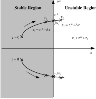
Fig -3: Illustration of roots of characteristic movement with respect to time delay

In the delay-dependent case, the roots of the characteristic equations move as the time delay



increases starting from 0. Figure 3 illustrates the movement of the roots. Note that the delay–free system (



0) is assumed to be

stable. This is a realistic assumption since for the practical values of system parameters the excitation control system is stable when the total delay is neglected [1]. Observe that as the time delay



is increased, a pair of complex eigenvalue moves in the left half of the complex plane. For a finite value of 0, they cross the imaginary axis and pass to the right half plane. The time delay value * at

which the characteristic equation has purely imaginary eigenvalues is the upper bound on the delay size or the delay margin for which the system will be stable for any given delay less or equal to this bound,   *. In order to

characterize the stability property of (4) completely, we first need to determine whether the system for any given set of parameters is delay-independent stable or not, and if not, to determine the delay margin * for a wide range

of system parameters.

In the following section, we present a practical approach that gives a criterion for evaluating the delay dependency of stability and an analytical formula to compute the delay margin for the delay-dependent case.

3. DELAY MARGIN COMPUTATION

A necessary and sufficient condition for the system to be asymptotically stable is that all the roots of the characteristic equation of the generator excitation control system with a stabilizing transformer, given in (4), lie in the left half of the complex plane. In the single delay case,

the problem is to find values of * for which the

characteristic equation of (4) has roots (if any) on the imaginary axis of the s-plane. Clearly, ( s, ) 0 is an implicit function of s and



which may, or may not, cross the imaginary axis. Assume for simplicity that ( s, 0)0 has all its roots in the left half plane. That is, the delay-free system is stable. Observe that the characteristic equation of (4) has an exponential transcendentality feature because of the term _es _{. This results in infinitely many} finite roots, which makes the determination of the roots and delay margin a difficult task. However, this problem could be easily overcome by using an exact substitution for the transcendental term suggested by Rekasius [14]. This substitution is given as;

1

,

1

s Ts

e T

Ts



_

 _  _ _

 (7)

and is defined only for s=jωc. It should be pointed out that

(7) is an exact substitution, not an approximation, when the characteristic equation of (4) has roots on the imaginary axis. Further, (7) gives the following mapping condition relating ωc and T [14, 16]:

1

2

* ( _c ) 0,1, 2,...

c

Tan T

  





 

 _  _  (8)

This equation describes an asymmetric mapping in which one T is mapped into infinitely many*’s for a given ωc.

Inversely, for the same ωc, one particular * corresponds

to one T only. The substitution of (7) into (4) results in a new characteristic equation as;

7 6 5 4

3 2

3 2 1 0

( , )

0

s T a s a s a s a s

a s a s a s a

     

    (9)

where

7 6 5 5 4 3 3 2 2

1 1 1 0 6 6 5 4 4 3

2 2 2 1 1 0 0

, , ( - )

- , ,

( - ) ,

a p T a p p T a p p q T

a p q q T a p p T a p p T

a p q p q T a q

    

     

   

(10)

This method reduces the stability problem effectively to one free of delay, which in turns requires calculating only roots of a single-variable polynomial. It is obvious from (9) that after Rekasius substitution the system characteristic equation of (4) has become an ordinary polynomial whose coefficients are parameterized in T only. Note that

T



,

thus it can also be negative. It must be noted that the 6th

order characteristic equation with delay given in (4) is now converted into a 7th_{order polynomial given in (9)}

[image:4.595.41.198.149.311.2]

(5)

Page 280

perfect coincidence with respect to the imaginary roots,

we prefer solving the simpler



(T_k,



_ck) for ( , ) s T 0



instead of



*



(_k_,_ck) for ( , ) s 0 . The question is to determine all T values, which causes imaginary roots

of s j_c of the augmented characteristic equation

( , )s T 0

  . For this purpose, Routh-Hurwitz criterion could be utilized. To determine the values of substitution parameter T, we need to form the Routh array based on (9) and set the only term R₁₁( )T in the s1 row to zero [16, 17, 23]. The Routh’s array is obtained as;

7

7 5 3 1

6

6 4 2 0

5

51 52 53

4

41 42 43

3

31 32

2

21 22

1 11

0 0

0 0 0

s a a a a

s R R R

s R R

s R

(11)

where

6 5 7 4 21 32 31 22

51 11

6 21

- -R

=a a a a ,..., =R R R

R R

a R

(12)

By setting the term R₁₁( )T in the s1 row to zero we obtain the following 14th_{order polynomial of}_T_as;

14 13

14 13 ... 1 0 0

t T t T  t T t (13)

The roots of this polynomial may easily be determined by standard methods. Depending on the roots of (13), the following situation may occur:

i) The polynomial of (13) does not have any real roots, which implies that the characteristic equation of (4) does not have any roots on the

j



-axis. In that case, the

system is stable for all



0, indicating that the system is

delay-independent stable.

ii) The polynomial of (13) has at least one real root, which implies that the characteristic equation of (4) has at least a pair complex eigenvalues on the j



-axis. In that

case, the system is delay-dependent stable.

The polynomial given by (13) may have at most fourteen real roots, T_c 



T T₁, ₂,....,T₁₄



. Once this set of real roots is

determined, the corresponding crossing frequencies c

s j can be found using the auxiliary equation, which

is formed by the _s2_{row of the Routh’s array. For a real}

i c

T T i1, 2,...,14, the auxiliary equation is given as

follows;

2

21( )c 22( )c 0

R T s R T  (14)

It must be mentioned here that in order for (14) to yield imaginary roots s j_c, the following additional condition has to be satisfied also [23];

21 22 0

R R  (15)

Observe that the coefficient R₂₁ is a function of T_c and

22

R is a positive constant coefficient since

22 0 G R A E I

R a K K K K K . For this reason, the auxiliary equation will yield imaginary roots, for positive R₂₁ only. For those T_c values, the crossing frequencies are obtained from (14) as;

22

21

( ) ( ) c c

c

R T

  (16)

Observe that we can determine at most fourteen different crossing frequencies



 c1, c2,...,c14



corresponding to



1, 2,...., 14



c

T  T T T . Substituting



_ci and T_i for

1, 2,...,14

i into (8), we can further get the corresponding

time delays



 ₁ , ₂,...,₁₄



. According to the definition of

delay margin, the minimum of those time delays will be the system delay margin.

4. THEORETICAL AND SIMULATION RESULTS

4.1 THEORETICAL RESULTS

In this section, the delay margin * for stability for a wide

range of PI controller gains is computed using the analytical procedure described in previous section. Theoretical delay margin results are verified by using Matlab/Simulink. The gains and time constants of the exciter control system used in the analysis are as follows [1]. K_A5, K_EK_G K_R1.0, K_F 2.0 T_A0.1 ,s

0.4 , 1.0 , 0.05 ,

E G R

T  s T  s T  s T_F 0.04 s.

First, we choose a typical PI controller gains

1

0.7; 0.8

P I

K  K  s to demonstrate the delay margin

computation. The process of the delay margin computation consists of the following four steps:

Step 1: Determine the characteristic equation of time delayed excitation control system using Eqs. (4) and (5). This equation is found to be:

5 6 5 4 3

2 2

( , ) (8x10 0.00468 0.4416 8.427

16.99 9.0 ) + (0.14 3.66 4) s 0

s s s s s

s s s s e 

 



     

(6)

Page 281

Step 2: Apply Rekasius substitution given by (7) into (4)

so as to obtain the new characteristic equation given by (9). The coefficients of this equation are found to be

7 6

5 4

3 2

1 0

0.00008 ; 0.00008 0.00468 ;

0.00468 0.4416 ; 0.4416 8.427 ;

8.427 16.85 ; 17.13+5.34

12.66 4 ; 4

a T a T

a T a T

a T a

  

   

  

  

Step 3: Compute elements of Routh table given by (12) and determine the values of T_c using (13). Only ten of the fourteen roots of (13) are found to be real. These real roots are given below.

1 2 3

4 5 6

7 8 9

10

1.61122; = 0.05242; 0.05240;

1.07826; 0.05320; 0.04569;

= 0.05006; 0.01709; 1.51469;

0.01698

T T T

T

   

     

    

 

Step 4: Compute R₂₁ for all T and check their sign. Note that for only T₁=1.61122, R₂₁ is positive and its value is

21 23.331

R  . For this reason, the remaining real roots T are not taken into account since they will not result in imaginary roots for the characteristic equation of the AVR system defined by (4) or equivalently the auxiliary equation given in (14).

Step 5: Compute the crossing frequency _c using (16) and the corresponding delay margin using (8). They are found to be _c0.414 rad/s and *2.8417 s. This result indicates that the delay margin is about _*__{2.8417 s}_for

0.7, P

K  K_I 0.8 s1. When time delay exceeds this

value, the generator excitation control system will become unstable.

Table -1: Delay Margins *for different values of KIand

KP of the AVR system with a stabilizing transformer

KI(S-1)

*

 (s) KP =

0.3 K0.5 P = K0.7P = K0.9P =

0.1 5.3902 4.4619 3.8120 3.4569

0.2 4.0139 3.8831 3.6424 3.4205

0.3 3.4744 3.4786 3.4050 3.2994

0.4 3.1986 3.2308 3.2159 3.1710

0.5 3.0347 3.0710 3.0775 3.0619

0.6 2.9275 2.9617 2.9760 2.9745

0.7 2.8527 2.8833 2.9000 2.9052

0.8 2.7978 2.8248 2.8417 2.8501

0.9 2.7561 2.7799 2.7960 2.8056

1.0 2.7234 2.7444 2.7594 2.7694

0 10 20 30 40 50 60 70 80 90 100

-1 -0.5 0 0.5 1 1.5 2 2.5 3

Time (s)

G

e

n

e

r

a

to

r

t

e

r

m

in

a

l

v

o

lt

a

g

e

V

t

(

p

u

)

  

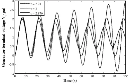
Fig -4: Voltage response of the AVR system with a stabilizing transformer for

K

_P



0 7

.

,

K

_I



0 8

. s

1and

three different time delays 2.74 , 2.876 , and 3.0 s s s

For the theoretical analysis, the effect of PI controller gains on the delay margin is also investigated. For this reason, different values of PI controller gains are selected, and the delay margin * is computed using the proposed method. Table 1 shows the complete theoretical results on the delay margins of the AVR system with a stabilizing transformer for the range of K_P0.3 0.9 and

1

0.1 1.0

I

K   s .

It is clear from the table that the delay margin decreases as the integral gain increases when K_P is fixed. Moreover, the comparison of delay margin results presented in Table 1 with those of the AVR system without a stabilizing transformer (see Table 2 in [19]) indicates that compensation of the AVR system by a stabilizing transformer significantly increases the delay margins for all values of PI controller gains, which makes the AVR system more stable. For example using the Rekasius substitution, for K_P0.7 and K_I 0.8 s1, the delay

margin when a stabilizing transformer not included is found to be  0.1563 s while it is  * 2.8417 s when a

[image:6.595.316.539.101.245.2]

(7)

Page 282

4.2 VERIFICATION THEORETICAL RESULTS WITH

MATLAB/SIMULINK

Matlab/Simulink is used to verify the theoretical results on the delay margin. For the illustrative purpose, PI controller gains are chosen as KP = 0.7, KI = 0.8 s-1. From

Table 1, for these gains, the delay margin is found to be 2.8417 s

 . However, the delay margin is found to be 2.876 s

 by using simulation. The error between the theoretical and simulation results for the delay margin is evidently negligible. It must be stated here that for theoretical computation of roots and delay margin, Mathcad program [24] is used, because this program is commonly used for cases in which extensive symbolic computations such as those presented in this paper are involved. On the other hand, time-domain simulation capabilities of Matlab/Simulink are utilized to verify theoretical delay margin results. It is possible that the usage of two different software packages, Mathcad and Matlab may result in such an error.

Simulation results for 2.876 s as well as two other delay values (



2.74 s and



3.0 s) are shown in

Figure 4. From the figure, it is clear that at 2.876 s_the sustained oscillations are occurred indicating a marginally stable operation. When the time delay is less than the delay margin ( 2.74 s), it is expected that the exciter system will be stable. On the other hand, when the time delay is larger than the delay margin, the system will have growing oscillations indicating an unstable operation, as illustrated in Figure 4 for



3.0 s. These

simulation results show that the Rekasius method correctly estimates the delay margin of the system.

5. CONCLUSIONS

This paper has proposed an exact method to compute the delay margin for stability of the AVR system including stabilizing transformer. The method first eliminates the transcendental term in the characteristic equation by using Rekasius substitution. With the help of this substitution, the characteristic equation has become a regular polynomial whose purely imaginary roots are the same as those of the transcendental equation. Routh stability criterion has been applied to determine the imaginary roots at which stability feature of the AVR system change and the corresponding delay margin.

The effect of PI controller gains on the delay margin has been investigated. The theoretical results indicate that the delay margin decreases as the integral gain increases for a given proportional gain. Such a decrease in delay margin implies a less AVR system. Moreover, it has been observed that the compensation of the AVR system with a stabilizing

transformer increases the delay margin of the system, which indicates a more stable AVR system.

Theoretical delay margin results have been verified using time domain simulations of MATLAB/Simulink. It has been observed that percentage error between the theoretical delay margin results and ones determined by simulation are negligible, which indicates the validity and effectiveness of the proposed method.

The following studies have been put in perspective as future work: i) the extension of the proposed method into multi-machine power systems with commensurate time delays; ii) the influence of power system stabilizer on the delay margin.

APPENDIX

The coefficients of polynomials

P s

( )

and

Q s

( )

given in

(5) in terms of gains and time constants of the AVR system:

6

5

4

3

( )

(

)

(

A E F G R

A E F G R A E F A E G A F G E F G

A E F A E G A F G E F G

R A E A F E F A G

E G F G A E P F G

A E A F E F A G E G F G

A E P F G R

p T T T T T

p T T T T T T T T T T T T T T T T T

p T T T T T T T T T T T T

T T T T T T T T T

T T T T K K K K T

p T T T T T T T T T T T T

K K K K T T



    

   

 

      



2

1

2

1

0

)

( 1)

1

( )

A E F A E P F

A E I F G G

A E F A E P F A E I F G G

R A E I F

A E I F

A E P G R F

A E G R P I F

A E I G R

T T T K K K K

K K K K T T

p T T T K K K K K K K K T T

T K K K K

p K K K K

q K K K K K T

q K K K K K K T

q K K K K K

   



      

  



 



REFERENCES

[1] H. Saadat. ‘Power system analysis.’ New York: McGraw Hill; 1999.

[2] P. Kundur. ‘Power system stability and control.’ New York: McGraw Hill; 1994.

[3] R. C. Schaefer and K. Kiyong. ‘Excitation control of the Synchronous generator.’ IEEE Industry Applications Magazine, vol 7, no 2, pp 37. 2001.

(8)

Page 283

[5] B. Naduvathuparambil, M. C. Valenti and A. Feliachi.

‘Communication delays in wide area measurement systems.’ The 34th_{Southeastern Symposium on}

System Theory ~SSST2002~, Huntsville, AL (USA), pp. 118, March 2005.

[6] X. Xia, Y. Xin, J. Xiao, J. Wu and Y. Han. ‘WAMS Applications in Chinese power systems.’ IEEE Power and Energy Magazine, vol 4, no 1, pp 54, 2006. [7] K. E. Holbert, G. T. Heydt and H. Ni. ‘Use of satellite

technologies for power system measurements, command, and control.’ Proceedings of the IEEE, vol 93, no 5, pp 947, 2005.

[8] J. Chen, G. Gu and C. N. Nett. ‘A new method for computing delay margins for stability of linear delay systems.’ System and Control Letters, vol 26, no 2, pp 107, 1995.

[9] K. Gu, V. L. Kharitonov and J. Chen. ‘Stability of time delay systems.’ Birkhauser; 2003.

[10]P. Fu, S. I. Niculescu and J. Chen. ‘Stability of Linear Neutral Time-Delay Systems: Exact Conditions via Matrix Pencil Solutions.’ IEEE Transactions on Automatic Control, vol 51, no 6, pp 1063, 2006. [11]K. E. Walton and J. E. Marshall. ‘Direct Method for TDS

Stability Analysis.’ IEE Proceeding Part D, vol 134, no 2, pp 101, 1987.

[12]J. H. Su. ‘The asymptotic stability of linear autonomous systems with commensurate time delays.’ IEEE Trans. Autom. Control, vol 40, no 6, pp 1114, 1995.

[13]J. Louisell. ‘A matrix method for determining the imaginary axis eigenvalues of a delay system.’ IEEE Trans. Autom. Control, vol 46, no 12, pp. 2008, 2001. [14]Z. V. Rekasius. ‘A stability test for systems with

delays.’ in Proceedings of Joint Automatic Control Conference, San Francisco(CA) Paper No. TP9-A, 1980.

[15]D. Hert, E. Jury and E. Zeheb. ‘Simplified Analytic Stability Test for Systems with Commensurate Time Delays.’ IEE Proceeding D- Control Theory and Applications, vol 131, no 1, pp 52, 1984.

[16]N. Olgac and R. Sipahi. ‘An exact method for the stability analysis of delayed linear time-invariant (LTI) systems.’ IEEE Trans. Autom. Control, vol 47, no 5, pp 793, 2002.

[17]N. Olgac and R. Sipahi. ‘A practical method for analyzing the stability of neutral type LTI-time delayed systems.’ Automatica, vol 40, no 5, pp 847, 2004.

[18]R. Sipahi and N. Olgac. ‘A comparative survey in determining the imaginary characteristic roots of LTI time delayed systems.’ in Proc. 2005 IFAC World Congress, Prague(Czech Republic), pp. 118, July 2005. [19]S. Ayasun and A. Gelen. ‘Stability analysis of a generator excitation control system with time delays.’ Electrical Engineering, vol 91, no 6, pp 347, 2010.

[20]H. J. Jia, X. D. Cao, X. D. Yu and P. Zhang. ‘A simple approach to determine power system delay margin.’ in Proc. 2007 IEEE Power Engineering Society General Meeting, Tampa, Florida (US), pp 1, June 2007.

[21]R. Sipahi and N. Olgaç. ‘Active Vibration Suppression with Time Delayed Feedback.’ Journal of Vibration and Acoustics, vol 125, no 3, pp. 384, 2003.

[22]MATLAB. ‘High-performance numeric computation and visualization software.’ The Mathworks; 2001. [23]K. Ogata. ‘Modern Control Engineering.’ Upper Saddle

River, NJ: Prentice Hall; 1997.

BIOGRAPHIES

Şahin Sönmez is currently working as a research assistant in the Department of Electrical and Electronics Engineering of Nigde University, Turkey. His research interests include modeling and stability analysis of power systems.

Ulas Eminoglu is currently working as an associateprofessor in the Department of Electrical Engineering of Nigde University,

Turkey. He has studied

distribution systems load flow analyses and power electronics, wind turbines.

Saffet Ayasun is currently working as a professor in the

Department of Electrical

An Exact Method to Compute Time Delay Margin for Stability of Time- Delayed Generator Excitation Control System

Page 276