Utilising the grid for augmented reality

(1)

Utilising the Grid for Augmented

Reality

Chris J. Hughes

A Thesis presented for the degree of

Doctor of Philosophy

High Performance Visualization and Medical Graphics

School of Computer Science

Bangor University

UK

(2)

Utilising the Grid for Augmented Reality

Chris J Hughes

Submitted for the degree of Doctor of Philosophy

January 2008

Abstract

Traditionally registration and tracking within Augmented Reality (AR) applica-tions have been built around specific markers which have been added into the user’s viewpoint and allow for their position to be tracked and their orientation to be es-timated in real-time. All attempts to implement AR without specific markers have increased the computational requirements and some information about the environ-ment is still needed in order to match the registration between the real world and the virtual artifacts. This thesis describes a novel method that not only provides a generic platform for AR but also seamlessly deploys High Performance Computing (HPC) resources to deal with the additional computational load, as part of the dis-tributed High Performance Visualization (HPV) pipeline used to render the virtual artifacts. The developed AR framework is then applied to a real world application of a marker-less AR interface for Transcranial Magnetic Stimulation (TMS), named BART (Bangor Augmented Reality for TMS).

(3)

iii

(4)

Declaration

The material in this thesis has not been previously submitted for a degree or diploma in any university. To the best of my knowledge this thesis contains no material pre-viously published or written by another person except where due acknowledgement is made in the thesis itself.

Chris Hughes

Date: 31st January 2008

(5)

Acknowledgements

• Prof. Nigel John, for without his support, ideas, encouragement and his

un-derstanding of my creative interpretations of his deadlines, this Thesis would never had existed.

• Dr. Franck Vidal, for not only having managed to share an oﬃce with me for

over 4 years, but mainly for the contribution of the word ’instead’ which he has kindly donated to page 80.

• Dr. Ade Fewings for pathing the way to >4 year PhD submissions. Also to

everyone else in the Graphics Group at Bangor University.

• Jason Lauder and Bob Rafal from the School of Psychology, Bangor University,

for allowing us access to their TMS laboratory and for supplying data from past experiments.

• The e-Viz teams at University of Manchester (Dr. John Brooke and Mark

Riding), University of Leeds (Prof. Ken Brodlie and Dr. Jason Wood) and Swansea University (Prof. Min Chen, Dr. Mark Jones, David Chisnall and Nicolas Roard) for their help and support.

• Ian Grimstead for his initial encouragement towards research in the field of

Visualization.

(6)

vi

• My Mum for encouraging me to follow my dreams and for not being

dissa-pointed when I turned out to be an academic.

• Chris Headleand and Sam Godwin, for giving me a much needed outlet for

my built up frustration and aggression by helping to bring the sport of Canoe Polo to Bangor. Also to the many people who have folloId in my footsteps to ensure there is always a game to play.

• The many authors and artists who have influenced me over the last 4 years,

particularly: Douglas Adams, Robert Rankin, Mark Thomas, Tenacious D.

• This research is supported by the EPSRC within the scope of the project: ”An

(7)

List of Abbreviations

AG Access Grid

ANL Argonne National Laboratory

API Application Programming Interface

AR Augmented Reality

ARToolkit Augmented Reality Toolkit

BART Bangor AR for TMS

CAVE Cave Automatic Virtual Environment

CoG Java Commodity Grid Kit

CRC Cyclic Redundancy Check

CSAR Computer Services for Academic Research

DART Designers Augmented Reality Toolkit

EPSRC Engineering and Physical Sciences Research Council

fMRI functional Magnetic Resonance Imaging

FPS Frames Per Second

(8)

viii

GGF Global Grid Forum

GPU Graphics Processing Unit

GRAM Grid Resource Allocation and Management

GSI Grid Security Infrastructure

GUI Graphical User Interface

HIT Lab Human Interface Technology Lab

LCD Liquid Crystal Display

HMD Head Mounted Display

HPC High Performance Computing

HPV High Performance Visualization

ICENI Imperial College e-Science Networked Infrastructure

IPG NASA’s Information PoIr Grid

IR InfraRed

JPEG Joint Photographic Experts Group

MR Mixed Reality

MVE Modular Visualization Environments

OGSA Open Grid Services Architecture

OGSI The Open Grid Services Infrastructure

(9)

ix

osgART open scene graph ARToolkit

PDA Personal Digital Assistant

PSE Problem Solving Environment

SDK Software Development Kit

SGS Steering Grid Service

skML skm Markup Language

SOA Service Orientated Architecture

SOAP Simple Object Access Protocol

TMS Transcranial Magnetic Stimulation

UnICoRe Uniform Interface to Computing Resources

V4L Video for Linux

VE Virtual Environment

ViPar Visualization in Parallel

VR Virtual Reality

VRML Virtual Reality Modelling Language

VTK Visualization Toolkit

WSRF Ib Services Resource Framework

WSDL Ib Services Description Language

(10)

List of Figures

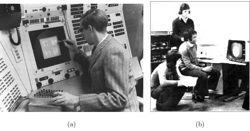
1.1 Early work at (a) MIT and (b) Bangor University, showing how users were able to interact with the early Computer Graphics applications. 1 1.2 (a) 1966: Ivan Sutherland’s CRT based HMD (b) Modern day: A

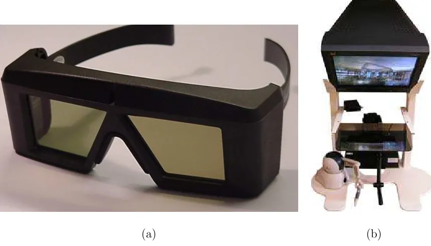
typical HMD with stereo capabilities up to 800x600 resolution. Com-mercially available for approx $5000. . . 3 2.1 An example of (a) a pair of Shutter Glasses from CrystalEyes and (b)

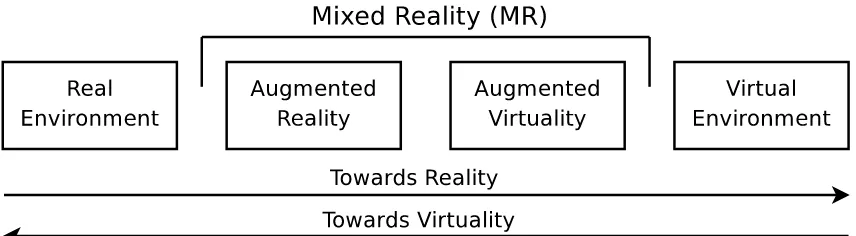
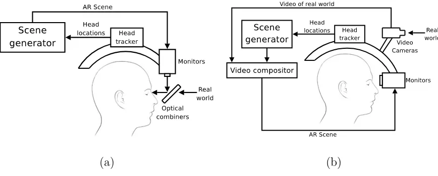
a desktop version of the Immersive Workbench from Sensegraphics. . 15 2.2 The basic set up of theCave Automatic Virtual Environment (CAVE) 16 2.3 Milgram and Kishino’s reality-virtuality continuum. . . 17 2.4 Comparison of (a) Optical through HMD and (b) Video

see-through HMD. . . 18 2.5 Examples of visualization work done at the School of Ocean Sciences

at the University of Wales Bangor: (a) The Lambeck European Ice Sheet and Shoreline 3D Visualisation Model and (b) The European Palaeotidal Visualisation Model. Images courtesy of A. Wainwright. . 26 2.6 Visualization Model: (a) The Computational cycle (b) The Analysis

cycle. . . 28 2.7 Haber and McNabb’s visualization model . . . 28

(18)

List of Figures xviii

2.8 Examples of Haptic devices: (a) Sensable Phantom Desktop, (b)

Sens-able Phantom Omni and (c) Novint Falcon. . . 31

2.9 Autonomic Computing deployment model. . . 43

3.1 A Biometric Analysis tool from Innovative Sports Training (IST). . . 50

3.2 The Wireless InertiaCube from Intersense. . . 52

3.3 (a) The Polaris Optical Tracking system and (b) a generic marker which will be used to track the electromagnetic coil. . . 53

3.4 The Polaris system emits IR light which reflects back from the mark-ers on each tool. . . 54

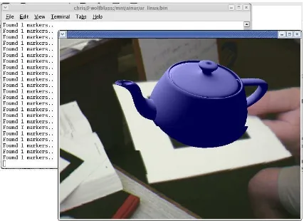
3.5 A virtual teapot is aligned with the real world using a marker detected by the ARToolkit. . . 56

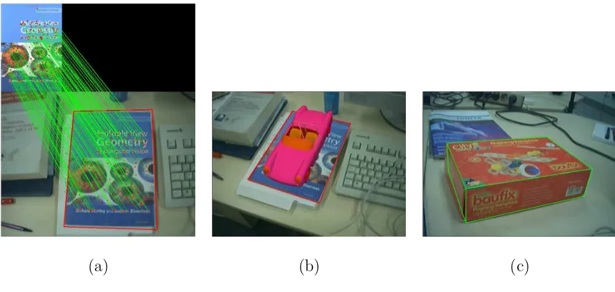
3.6 Three common methods for Pose Estimation: (a) Point-based, (b) Contour-based and (c) Texture-based. . . 59

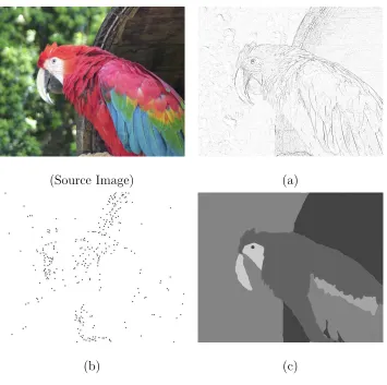
3.7 The three main categories of feature points: (a) Edge points, (b) Corner points and (c) Area points. . . 61

3.8 The steps involved in feature detection. . . 62

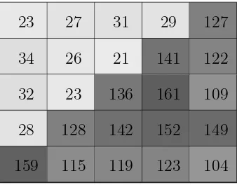
3.9 A subset of a grey-scale image showing an obvious edge. . . 62

3.10 Timeline of Corner Detectors. . . 64

3.11 The eight positions shifts required to calculate the intensity variation of the centre point. . . 65

3.12 The Moravec Operator used to extract corner points from a spinning cube, with some obvious points missed and circled in red. . . 66

(19)

List of Figures xix

3.14 The Web Service Concept. . . 69 3.15 The EuroGrid Project established a grid of resources from centres in

diﬀerent European countries. . . 78 3.16 The user’s of Grid based Visualization can be broken down into these

four groups. . . 82 3.17 An example of the RAVE client running on (a) A Linux PC (b) A

Windows CE based PDA, where both clients are connected to the same visualization. Images courtesy of Ian Grimstead, Cardiﬀ Uni-versity. . . 84 3.18 An OpenGL demonstration is distributed with Chromium (a) across

16 desktop computers and (b) tiled across a 2x2 display. Images courtesy of Ade Fewings. . . 85 3.19 The gViz reference model for describing visualization tasks. . . 87 4.1 A typical electromagnetic coil (a) and the magnetic field generated

(b) as used for TMS. . . 91 4.2 (a)The tracker used to identify the position of the subjects head, and

(b) The Brainsight software displaying targetting information on a computer display. . . 93 4.3 The tools being tracked: (a) The subjects head, The electromagnetic

coil and (b) the viewpoint of the operator captured using a webcam aligned with the digitizing probe . . . 94 4.4 System Diagram showing the flow of data and the tools that are being

tracked. . . 95 4.5 The virtual Camera, which is aligned with the real camera from the

(20)

List of Figures xx

4.6 The Calibration oﬀset for both the Camera C and the subject’s head

H need to be calculated. . . 100 4.7 The relationshipC between the Digitizing Probe and the camera lens

is calculated using a static point as a reference. . . 101 4.8 The transformation is calculated between the actual position of the

coil and the target position of the tool. . . 102 4.9 The OpenGL Targeting interface guides the operator to align the

magnetic coil with the desired region of interest. . . 104 4.10 The VTK rendering pipeline. . . 105 4.11 The composited operator’s view showing a visually acceptable

align-ment of the real world and the computer graphics . . . 105 5.1 The software layers for Computer Vision . . . 109 5.2 The Calibration tool allows the user to align a virtual object with an

object in the real world. . . 110 5.3 An example set of Haar-like features. . . 112 5.4 The cascaded Haar-classifier is presented with subsections of the

op-erator’s viewpoint. The subsection propagates through each classifier until either it passes each stage or it fails a single classifier, at which point the subsection is immediately rejected. . . 113 5.5 Multiple cascaded classifiers are used in parallel in order to identify

the source of the subsection from each of the diﬀerent calibrated views.114 5.6 The POS algorithm maps the 2D feature points from the operator’s

(21)

List of Figures xxi

5.8 A frame from our evaluation video, showing which calibration image has been used and some of the feature points that have been matched to it, whilst calculating the pose. . . 117 5.9 The weighting that classifier (1) allocated to each image of the test

video. . . 118 5.10 The weighting that classifier (2) allocated to each image of the test

video. . . 120 5.13 This graph shows the time take to process each frame of a

pre-recorded video stream. . . 120 6.1 The functional description of the e-Viz framework. Each of the coloured

components relates to its appropriate level of the same colour in Fig-ure 2.9. . . 124 6.2 The three components of the e-Viz framework. . . 126 6.3 The standard e-Viz client providing a Launcher application with a

vi-sualization wizard, and a remote Vivi-sualization viewer. Here a volume visualization of a hydrogen molecule is being rendered. . . 127 6.4 The Abstract Visualization Description Language allows a single

visu-alization task to be rendered using diﬀerent Visualisation applications - in this example AVS explorer (left) and VTK (right). . . 130 6.5 The e-Viz demonstrator using the ARToolkit to steer a simple

(22)

List of Figures xxii

6.6 Using e-Viz to remotely render a simple cone using VTK: (a) The simple ARToolkit based client used to steer the simulation and (b) the remotely rendered cone is displayed on the client. . . 134 6.7 The first grid enabled version of BART, uses e-Viz to perform the

remote rendering. . . 135 6.8 A typical MRI dataset used by BART (a) and the cranium segmented

from the dataset (b). . . 136 6.9 The second Grid enabled version of BART extends the pose

track-ing and estimation onto remote High Performance Computtrack-ing (HPC) resources as part of the e-Viz visualization pipeline. . . 138 6.10 The average time taken by each component of BART v3.1. The data

has been rounded for illustration purposes. . . 139 6.11 The distributed nature of the BART v3.1 system allows staggered

processes to be overlaid. . . 141 6.12 This graph shows the time between each frame of our test video that

is returned to the user. . . 142 7.1 The BART v1 software showing two of the operator’s views: (a) The

targeting tool helping to align the coil with a region of interest the subjects cranium and (b) a rendered view allowing the operator to see inside the subjects head. . . 147 7.2 The pose tracking and estimation from BART v2. . . 149 7.3 This graph shows the time between each frame of our test video that

is returned to the user. . . 150 7.4 Summary of the contribution towards evaluating the hypothesis

(23)

Chapter 1 Introduction

[image:23.612.114.551.332.562.2]

(a) (b)

Figure 1.1: Early work at (a) MIT and (b) Bangor University, showing how users were able to interact with the earlyComputer Graphics applications.

Since the TermComputer Graphicswas first coined in the early 1960’s by William Fetter to describe his work at Boeing [1], there has been a constant challenge not only to improve the quality of the computer graphics but also to find more natural interfaces between theComputer Graphics image and the real-world. Initially

(24)

Chapter 1. Introduction 2

ode ray-tube (CRT) monitors were the only technology that was available to display the computer output, however as computing resources became more powerful allow-ing Computer Graphics to improve, there was also a requirement to improve the methods by which users view the images.

Even in the early days it was clear how powerful the computer graphics could be. Figure 1.1, gives examples of some of the first computer graphics research being done, both at (a) MIT and at (b) Bangor University. Work done in 1965 by Ivan Sutherland produced the first Head Mounted Display (HMD) as a ‘window into a virtual world’, allowing the users to look into an environment that was completely computer generated and although the Computer Graphics were extremely basic it was a major milestone in the work towards immersive visualization environments [2]. However it was not until 1989 when Jaron Lanier used the phrase Virtual Reality (VR) and created the first commercial business around virtual worlds [3].

Twenty years later researchers are still working towards that goal. Computa-tional resources are much faster, most people have watches with more processing power than was available to them in the 1960’s and over 67% of all homes have a computer with the capabilities to generate real-time, photo-realistic environments. Ivan Sutherland’s CRT based HMD has now been replaced by ultra thin LCD dis-plays, but work is still going on to develop better and more natural ways to allow the user to understand the computer graphics.

(25)

Chapter 1. Introduction 3

(a) (b)

Figure 1.2: (a) 1966: Ivan Sutherland’s CRT based HMD (b) Modern day: A typical HMD with stereo capabilities up to 800x600 resolution. Commercially available for approx $5000.

for AR: a) the real and virtual world must be combined, b)the environment must be interactive whilst maintaining real-time performance (i.e. more than 15 frames per second) and c) the Computer Graphics must be registered in 3D [5].

(26)

1.1. Hypothesis 4

1.1 Hypothesis

The hypothesis is that it is possible to create an interactive Augmented Reality interface, using feature points for registration. It will also be capable of providing high performance visualizations by seamlessly deploying processing power from a remote, possibly Grid-enabled, high performance computing resource.

The framework developed will be applied to Transcranial Magnetic Stimulation.

1.2 e-Viz Project

The e-Viz project was funded by the EPSRC between November 2003 and Febru-ary 2007 to provide a solution to theGrand Challenge problems which require High Performance Visualization (HPV) resources. It was a collaborative project involving computer science groups at Bangor, Leeds, Manchester and Swansea Universities. By exploiting Grid technologies, e-Viz provides a generic flexible infrastructure for remote visualization allowing the rendering of large datasets whilst providing real-time, high resolution performance. It does this using a combination of intelligent scheduling for new rendering pipelines and the monitoring and optimisation of run-ning pipelines, all based on information held in a knowledge base. This provides an adaptive visualization service that provides rendered graphics reliably without the application or user even being aware of what resources are being used. An overview of the e-Viz framework is given in chapter 2.

(27)

in-1.3. Motivations of this work 5

tegrated into a Grid infrastructure and the application of autonomic computing strategies to visualization tasks - this is the first time that such a strategy has been proposed. Bangor’s contribution to the e-Viz project included the study of the performance of distributed graphics pipelines in a visualization architecture built on commodity PC hardware. This reflects the trend of incorporating such architectures in Grid computing, in place of supercomputers. Furthermore, the development of an augmented reality interface for transcranial magnetic stimulation using high per-formance computing resources, was created as an exemplar application for the e-Viz framework. The work of which is included as part of this thesis and is explained on more detail in Chapter 6.

1.3 Motivations of this work

Augmented Reality (AR) provides the user with the ability to visualize and project 3D data or other information into their natural environment. It also provides the user with an intuitive method of interacting with the data in a way that has not previously been available. By providing the user with an egocentric view of the visualized data allows them to use their natural spatial understanding and to gain a sense of their presence in the real world, augmented with virtual artifacts.

(28)

1.3. Motivations of this work 6

as a mobile phone, many of which have camera facilities built in.

The ability to visualize and interact with an environment that has been aug-mented with complex virtual artifacts could have a great impact upon many appli-cations. Some examples of these include:

Medical: During medical diagnostics or surgery, previously derived tomography could be overlaid over the patient allowing the clinician to ‘see’ inside the patient.

Manufacturing and Assembly: Assembly instructions could be placed into the field of view of the assembly worker.

Visualization of Architecture: Destroyed historic buildings could be virtually rebuilt, or planned construction projects be simulated.

Collaboration: Meetings could combine both real and virtual participants. Also a single 3D artifact could be explored by user’s from multiple locations.

(29)

1.4. Contributions of this research 7

• Must be easy to calibrate oﬄine which real world objects are being tracked. • Needs to be capable of automatically reinitializing should the alignment drift

or an error occur.

• Needs to extract feature points reliably and repeatably.

• Must have a computational cost that can be satisfied in real-time. • Must provide an accurate alignment of the virtual and real objects.

• Must work in unconstrained environments, such as changing levels of light. • must be able to be adapted for each required application.

The main challenges of this research include:

• Implementing a robust, repeatable feature point detector.

• Registering extracted feature points to a calibrated reference frame.

• Implementing a pose estimation algorithm in order to reconstruct the position

and orientation of the tracked object.

• Utilise the e-Viz framework to seamlessly deploy the computational load of

the AR application to a remote Grid enabled resource.

• Attempt to achieve an Autonomic AR environment with support for

Self-configuration, Self-healing, Self-optimization and Self-protection.

1.4 Contributions of this research

(30)

1.4. Contributions of this research 8

more computationally intensive AR environments to be generated. Specifically the contributions include:

• A novel AR interface to theTranscranial Magnetic Stimulation (TMS) using

aPolaris Optical Tracking System was developed. This allows the operator to identify and align the TMS tools with the required regions of interest on the subject’s cranium, whilst working in a much more natural environment. The software,Bangor Augmented Reality for TMS (BART) allows the operator to see the actual rendering of the subjects cranium whilst interacting with the subject rather than focusing at a computer monitor.

• A new framework for tracking, using only a cheap webcam rather than an

expensive proprietary tracking system was developed. By extracting feature (or corner) points from the user’s viewpoint the software is able to track the position and pose of the real world object that was used for reference. A Haar-classifier technique was combined with a POSIT algorithm to track the position of the moving object and calculate its change in orientation and rotation within set error bounds.

• In order to use BART in real-time with large volume datasets, the e-Viz

frame-work was successfully used to transparently allocate a remote High Perfor-mance Visualization (HPV) resource to remotely render the virtual artifacts.

• To satisfy the large computational requirements of the BART software it was

finally distributed as part of the visualization pipeline. The e-Viz framework was used to allocate remoteHigh Performance Computing (HPC) resources.

• During this research a significant contribution was made to the development

(31)

1.5. Publications 9

outstanding by the EPSRC reviewers. Specifically, contributions were made to the following components of e-Viz included:

– Contribution to the overall system design.

– Development and maintenance of the e-Viz broker and database which ran on a machine based at Bangor.

– Development of an e-Viz wrapper for openDX, allowing it to be used as a remote visualization software resource.

– Install and testing of the e-Viz software during development.

1.5 Publications

The following publications where contributed to during this research project:

1.5.1 Journal Publications:

(1) K Brodlie, J Brooke, M Chen, D Chisnall, A Fewings,C Hughes, N.W. John, M Jones, M Riding, and N Roard, ‘Visual Supercomputing - Technologies, Applications and Challenges’, Computer Graphics Forum, Number 24, Issue 2, pp. 217-245, 2005.

1.5.2 Publications in refereed conference Proceedings:

(32)

1.5. Publications 10

(3) C. J. Hughes, N. W. John, ‘A generic approach to High Performance Visu-alization enabled Augmented Reality’, Proceedings of Theory and Practice of Computer Graphics, Bangor, pp. 181-186, ISBN 978-3-905673-63-0, 2007. (4) Chris Hughes and Nigel W. John, ‘A flexible infrastructure for delivering

Augmented Reality enabled Transcranial Magnetic Stimulation’, Proceedings of Medicine Meets Virtual Reality 14, Long Beach, California, pp. 219-224, IOS Press, ISBN 1-58603-583-5, 2006.

(5) Mark Riding, Jason Wood, Ken Brodlie, John Brooke, Min Chen, David Chis-nall, Chris Hughes, Nigel W. John, Mark W. Jones, Nicolas Roard, ‘e-Viz: Towards an Integrated Framework for High Performance Visualization’, Pro-ceedings of the UK e-Science All Hands Meeting, EPSRC, pp. 1026-1032, ISBN 1-904425-53-4, 2005.

(6) K. Brodlie, J. Brooke, M. Chen, D. Chisnall, A. Fewings, C. Hughes, N.W. John, M. Jones, M. Riding, and N. Roard, ‘Visual Supercomputing - Technolo-gies, Applications and Challenges’, STAR Report, Eurographics, Grenoble, France, 2004.

1.5.3 Refereed Poster Presentations:

(7) K. W. Brodlie, J. Brooke, M. Chen, D. Chisnall, C. J. Hughes, N. W. John, M. W. Jones, M. Riding, N. Roard, M. J. Turner and J. Wood, ‘A Frame-work for Adaptive Visualization’, Poster presentation for IEEE Visualization, Baltimore, Maryland, USA, 2006. Poster presented by Hughes.

(33)

1.5. Publications 11

at UK e-Science Programme All Hands Meeting, Nottingham, 2006. Poster presented by Hughes.

1.5.4 Summary of contribution to each publication:

Paper (1) was a revision of Paper (6) which was originally drafted as the literature review for this thesis. It was moderately redeveloped, as a state-of-the-art report with contributions from the e-Viz consortium. Paper (2) summarises the final results of the e-Viz project. Paper (3) detailed the BART v3 software, as shown in Chapter 6, and how it was integrated to use the e-Viz framework. Paper (4) was based upon the first version of BART as described in Chapter 4. Paper (5) described the design of the e-Viz system, including details about the Broker web service.

(34)

Chapter 2 Background and Literature

Review

2.1 Virtual Environments

Virtual Environments represent a major technical drive in computer graphics and visualisation, and have helped push a range of hardware and software technologies forward. A Virtual Environment (VE) gives the user a feeling of being inside a com-puter generated environment with a sense of spatial presence and often coupled with physical presence. For many visualisation applications, Virtual Environments can provide user’s with realistic experience in interrogating, navigating within, feeling and manipulating data via its visual representation.

The visual display can be broken down into three diﬀerent types of immersive display. These three types are described below:

(35)

2.1. Virtual Environments 13

2.1.1 Non-Immersive Displays

The most basic method of stimulation is to use a computer display to show the user graphics information, allowing the user to view the the virtual environment through a window. Generally these environments allow the user to interact using a mouse or a keyboard. However using an ordinary computer display has many limitations and the user would only see a flat image and do not give the user a true feeling of being immersed within the virtual environment. To try and extend upon this scientists have developed several ways to send a diﬀerent image to each eye and thus give the user a 3D perspective of the image.

2.1.2 Semi-Immersive Displays

One popular method is to use active-stereo and Shutter Glasses, as shown in Fig-ure 2.1(a). With this technology an ordinary computer monitor can be used and allow several people to view the visualization at a time. These work by using LCD panels to alternatively block the light to each of the user’s eyes. This can then be synchronized to the monitor which can display diﬀerent projections for each eye by switching between the images very quickly [6]. These allows the user to get a true grasp of the 3D environment and although the user can still see the real world around them, gives them a more realistic view of the objects and environment into which they are looking. There are several commercial versions of the Shutter Glasses from companies such as CrystalEyes [7] and StereoGraphics [8].

(36)

cheaply. The image is projected from two digital projectors with their image filtered to match the separate polarization filters in the viewer’s glasses. This means that each eye can only see the image from one of the projectors and therefore the stereo image can be produced by sending a diﬀerent projection to each eye.

Auto-stereoscopic displays are being developed to enable the user to see into the virtual environment in 3D without the need for Shutter Glasses, such as the SeeReal display from inition [10]. However many of these displays can be diﬃcult to set up successfully and require the user to be sit in a specific position, making it diﬃcult for collaborative use.

Another example of semi-immersive displays is the Immersive Workbench from Sensegraphics [11]. They have developed an environment which uses a standard computer display, which is reflected from a semi-transparent mirror. This allows the user to look down into the virtual environment through the mirror using Shutter Glasses. This allows the user to not only see the 3D environment, but also leaves the real workspace within the environment empty for other tools to be used, such as Haptic devices which allow the user to touch the objects within the environment. The Immersive Workbench is available in a number of diﬀerent formats, ranging from the desktop version, as shown in Figure 2.1(b) using a CRT monitor, up to a collaborative version using a 3D digital projector to provide a much bigger working environment.

2.1.3 Fully-Immersive Displays

(37)

[image:37.612.114.544.102.347.2]

(a) (b)

Figure 2.1: An example of (a) a pair of Shutter Glasses from CrystalEyes and (b) a desktop version of the Immersive Workbench from Sensegraphics.

see the visualization at once, but it did ensure that the user would only be able to see the computer environment. This provides a number of other limitations such as the headsets were generally uncomfortable due to their size and weight. They also the user requires some form of cabled connection to the computer which could be cumbersome [12].

(38)

2.2. Augmented Reality 16

are available. Fakespace Systems [14] are one of the leading suppliers of immersive displays.

Figure 2.2: The basic set up of the Cave Automatic Virtual Environment (CAVE)

2.2 Augmented Reality

Augmented Reality (AR), is an extension of existing Virtual Environments (VE) which completely immerse a user inside a computer generated environment. By contrast, AR allows the user to see the real world, whilst supplementing it with virtual objects that are superimposed within the real world [5].

Milgram and Kishino’s continuum, shown in Figure 2.3, illustrates the diﬀerence between reality and virtuality with several steps between them. They define any step between the real world and a completely virtual environment as Mixed Reality (MR). In Augmented Virtuality real world views or objects are inserted into a virtual scene, rather than in AR where virtual objects are inserted into real world scene.

(39)

[image:39.612.107.535.96.214.2]

applica-2.2. Augmented Reality 17

Figure 2.3: Milgram and Kishino’s reality-virtuality continuum.

tions, including: medical visualization, maintenance and repair, annotation, robot path planning, entertainment and aircraft navigation [5].

2.2.1 Displays

Most AR technologies have been based upon the use of some form of transparent display which is positioned between the real world and the eyes of the user [15]. In order to align the computer graphics with the physical reality, cameras are used to track the movements of the user’s vision and allow the graphics to be realigned [16]. It is also possible for a collaborative AR in which several users can be tracked and see the same virtual objects from diﬀerent perspectives [17].

This can be done most simply using a HMD which is designed to allow the user to ‘see-through’ an optical combiner and therefore to be able to see the real world as well as the computer graphics as shown in Figure 2.4(a). Other HMD solutions include video see-through HMD’s which use dual cameras (to capture the real world in stereo) as shown in Figure 2.4(b). The video streams captured by these cameras is then composited with the computer graphics to generate the user’s view.

(40)

2.2. Augmented Reality 18

[image:40.612.114.548.97.272.2]

(a) (b)

Figure 2.4: Comparison of (a) Optical see-through HMD and (b) Video see-through HMD.

is usually done by the emission of a light source such as a laser into 3D space. Actuality Systems Inc, produce an auto-stereoscopic device which allows users to walk around and see a life size 3D image. It works by projecting a series of 2D images onto a rotating screen. Although this allows many people to look at the virtual objects simultaneously, it is very restrictive as the 3D objects can not be positioned arbitrarily into the real world.

2.2.2 Applications

(41)

2.3. High Performance Computing and the Computational Grid 19

This data can then be rendered in real time and overlaid onto the patient allowing the doctor virtually to see inside the patient [19].

The Eurographics Association, sponsor an annual medical prize, acknowledging research utilizing computer graphics within the medical field [20]. In 2003 the prize went to an AR application for Liver Surgery Planning, which utilized a Personal Interaction Panel (PIP) and a tracked pen to allow doctors to examine a patients liver. The PIP was used to allow doctors to specify cross sections of the liver that they wanted to examine.

Larose used a Tile system to create a PIP which was a two handed pen and pad interface into AR applications as part of the Studierstube AR Project [17] This panel allowed user’s to interact with virtual controls overlaid onto the panel.

2.3 High Performance Computing and the

Com-putational Grid

‘High Performance Computing (HPC) involves the use of parallel computing systems to solve computationally intensive applications’ [21].

(42)

There is a lot of research into the field of parallel algorithms, with a particular focus on developing algorithms which can provide scalability to perform eﬃciently depending upon the available resources.

Parallel architectures have also become very popular due to the eﬃciency that can be achieved at low cost. For example, it is possible to achieve the same level of processing power by using a number of cheap, desktop computer processors as you could from one expensive specialist processor [22].

There is no completely satisfactory way to characterize the diﬀerent types of parallel system. Flynn [23] devised a taxonomy that is still the most popular and widely used today. Streams of information are used to as the basis of classification. The streams of data that are received by a processor can be separated into two separate groups; instructions and data. Flynn’s taxonomy classifies each node in a parallel system according to whether it has one or more streams for each type of information.

2.3.1 Single Instruction, Single Data Stream (SISD)

This is the traditional uniprocessor model, where only one instruction can be exe-cuted at a time. This means that it is not possible to achieve parallelism, although it can closely be emulated by multitasking. This means that each process shares the processor usually on a time share basis.

2.3.2 Single Instruction, Multiple Data Streams (SIMD)

(43)

in sync. This global synchronization is generally performed by hardware. SIMD machines are particularly useful for processing vectors or images, where the data can be partitioned into separate blocks.

2.3.3 Multiple Instruction, Single Data Stream (MISD)

There are very few machines which would fit into this category, certainly none which have been particularly successful or had any impact on computer science. To construct an MIMD system several instructions streams would need to operate on the same data simultaneously. One example of an MISD machine is the experimental Carnegie-Mellon computer from 1971.

2.3.4 Multiple Instruction, Multiple Data Streams (MIMD)

This is the most general and most powerful model for high performance computing. Execution on each processor can be either synchronous or asynchronous, determin-istic or non-determindetermin-istic, running its own individual set of instructions on its own set of data.

It is possible to construct an MIMD machine using simple of the shelf processors, which are cheap and easily available. There are also a variety of remote message passing software systems available to allow the use of workstations on a network as MIMD systems.

2.3.5 Other Taxonomies

(44)

and how they are connected to the shared memory. Since these characteristics can have such a dramatic eﬀect on the performance of the system it would be more suitable to classify them diﬀerently.

A popular solution to this has been to extend the SIMD category to Single Program Multiple Data stream (SPMD) as it allow processing similar to SIMD on MIMD hardware. It is commonly used for trivially parallel problems such as queueing [24].

2.3.6 Example of a Parallel System

The University of California, Berkeley has a research department which is looking into more advanced techniques for analysing radio transmissions received by the Arecibo telescope in Puerto Rico. Their main project is called ‘The Search for Ex-traterrestrial Intelligence’ (SETI) and involves a number of mathematical functions which look for correlations in the received radio data.

Each day about 36Gb of data is recorded and has to be analysed. In order to do this however would require a large amount of very expensive processors. The team at Berkeley realized how much processor time was being wasted by privately owned computers sitting idle and realized that all of these computers could be utilized in the search for extraterrestrial transmissions.

In 1996 the idea for SETI@Home was first conceived that a screen saver could be released to the public which would be able to request small chunks of the data and perform the analysis on the data when the computer was idle. Finally in 1999 the software was released to the public. A lot of media attention launched the project and soon many computer user’s where keen to do their bit and to be involved.

(45)

2.4. High Performance Visualization 23

hosted at Berkeley. The server then sends back 0.25Mb of data to the client and keeps a record of where the processing is taking place. Once the data segment is processed which can take several hours, the result is returned to the server which correlates all of the results back together. If for any reason the server doesn’t receive a reply within a specified period the segment of data is simply sent to a diﬀerent client.

The SETI@Home project is an example of how supercomputer power can be achieved without the need to buy expensive mainframe computers. Now with nearly 4.5 million user’s there is the potential for millions of nodes to be running in parallel. To put this into perspective the SETI@Home website tells us that the most powerful computer, IBMs ASCI White, is rated at 12 TeraFLOPS and costs $110 million. SETI@home currently gets about 15 TeraFLOPs and has cost $500K so far [25] [26].

2.4 High Performance Visualization

High Performance Visualization (HPV) is the combination of the very latest visual-ization techniques along with the utilvisual-ization of High Performance Computing (HPC) resources.

(46)

2.4.1 Visualization

The basic aim of visualization is to convert a subset of data into a more perceptually understandable form by using computer graphics to represent the data.

The technique of visualization was around long before computers. Early scientists where forced to record their data using hand drawn images and diagrams to represent the information. This would have been a painstaking task and meant that early researchers had to be accurate artists as well as scientists [28].

With the progresses in technology users are now able to generate vast quantities of numerical data during our work or research. This can be achieved in many diﬀerent ways, including: computational simulations and actual measured data.

In order to implement visualization solutions it is necessary to find a method of presenting the original data into a graphical way that will be useful to the researcher and there are many trade-oﬀ’s that will have to be made to find the most eﬃcient method. Most of the current limitations with visualization are caused by the physical limitations of the computer systems being used. For example memory limitations may mean that the computational process will only be able to handle a small subset of the data at one time or the processing capabilities may mean that the computer system isn’t capable of processing the graphics in real time.

(47)

his movements. Then this path could be retraced later and an animation rendered over a longer period of time.

When the entire view of a dataset is rendered it is known as a qualitative overview but when a specific subset of the data is being represented then it is known as a quantitative study [28].

It is important to remember that although the process of visualization is a trans-formation from numerical data to computer graphics, the mapping is most likely to be a one way process and trying to recreate the original dataset from the visualiza-tion, could be impossible. It is also important to remember that the visualized data can be potentially inaccurate and is open to human interpretation and perception.

Generally before a dataset can be used, it is necessary to perform some filtering to prepare and clean up the data. Such as interpolating missing data values, removing noise and clamping data to specific ranges.

It is often desirable within a visualization to show a realistic representation of what the data represents, such as modelling prototypes or architectural based data. However it can be more useful to have a simplified representation which could be just as accurate. Other techniques for improving visualization include adding colour and motion.

(48)

Iteration is an important aspect of visualized data that changes over time and actually allows the researcher to manipulate the data using the process of steering, whilst actually seeing the eﬀects in real time.

Figure 2.5 shows two examples of visualizations being done at Bangor University. Figure 2.5(a) shows a model of the Lambeck European Ice Sheet. The model is being used to create a detailed reconstruction of the glacial movements over the last 10 years, with the aim of better understanding about glaciation and the underlying geology [29]. The European Palaeotidal Visualisation Model, shown in Figure 2.5(b) shows an example of where visualization is being used to predict tidal statistics based upon up to date palaeoshorline data [30].

(a) (b)

(49)

2.4.2 Visualization Model

Craig Upson, suggests that in order to ‘deal with the problems of multiple disciplines in the computational sciences eﬀectively, it is useful to begin by developing a coherent picture of the various steps a scientist takes while simulating a natural process using a computational model’ [31].

This simplifies to identifying the similarities between each discipline. Figure 5, demonstrates the process of numerical simulation using a computer program. It shows a circular path which can be repeated many times before a program is finely enough resolved.

The basic strategy to the computational cycle is that after the researcher has performed his initial research, he is ready to program an implementation. This implementation will then produce data which can be analysed. The outcome of this data will decide whether the researcher needs to return to the programming stage, or whether the implementation has succeeded.

The analysis step within the cycle can be broken down into the cycle shown in Figure 2.6(b). This shows that there are several main steps to the analysis of the data [31].

(50)

(a) (b)

Figure 2.6: Visualization Model: (a) The Computational cycle (b) The Analysis cycle.

Figure 2.7: Haber and McNabb’s visualization model

2.4.3 Human Factors involved in Visualization

Visualization really ‘attains its power by captivating the user’s attention by inducing a sense of immersion and presence’ [6]. This is achieved by using hardware that is able produce stimulations to the main senses of the human body, giving the user a feeling that they are immersed within the virtual environment [33].

(51)

2.4.4 Vision

The Human eye contains a lens which focuses the light on the light-sensitive retina at the back of the eyeball. The light information is then transferred via the optic nerve to the visual cortex [28].

The Human body has Stereoscopic vision. This means that by using two eyes the brain is able to estimate depth by the use of binocular disparity and ultimately gives rise to the sense of 3D vision by providing two diﬀerent images.

This is the most commonly stimulated sense, which is generally stimulated with the use of a video display which presents the visual information to the user.

Using an ordinary computer display has many limitations, as the user would only see a flat image. To try and extend upon this scientists have developed several ways to send a diﬀerent image to each eye and thus give the user a 3D perspective of the image.

2.4.5 Sound

The second sense is that of hearing. Human ears allow sound waves to be interpreted by conducting vibrations in the inner ear. The Human ears are also used to tell whether the body is standing upright, or leaning at an angle as well as identifying whether it is stationary or accelerating.

Motion sickness is caused when equilibrium is lost between all of the senses. For example if a person’s sight is telling him that he is moving, but his ears say that the body is stationary, then motion sickness can occur. This is an issue that can occur when immersed in a visualization environment, and must be considered.

(52)

used to simulate the appropriate environmental sound, it can add a great deal of realism when interacting with a visualized environment.

2.4.6 Haptics

Touch is also a very important sense. The human body is made up of a vast quantity of nerves which provide complex feedback from all over the human body. This allows the user to use their hand to actually feel the shape of objects and to identify different attributes such as texture and temperature. This is the most difficult sense to try and stimulate simply because it is very difficult to make it feel like you are actually touching an object without limiting the user’s capabilities [34].

The most eﬀective method for giving the user the impression of physically inter-acting with objects, is to use a Haptic Force Feedback Device such as the Phantom Desktop from SenseGraphics, as shown in Figure 2.8(a). Force Feedback Devices work by allowing the user the ability to freely use a stylus or joystick. However this stylus is fixed to a base and the computer has the ability to provide force back onto the device and depending upon the force used this can produce the feeling of resistance and create the feel of solid objects and diﬀerent textures.

Lower cost Haptic devices such as the Phantom Omni, as shown in Figure 2.8(b) have been developed in order to make the technology more readily available. Re-cently a domestic version, the Novint Falcon, has been released to meet the demand of the home gaming industry, shown in Figure 2.8(c).

(53)

(a) (b) (c)

Figure 2.8: Examples of Haptic devices: (a) Sensable Phantom Desktop, (b) Sens-able Phantom Omni and (c) Novint Falcon.

users.

2.4.7 Input Devices

The user also needs the facility to allow him to interact with the visualization in some way. There are several commercially available solutions to this.

The first is a 3D mouse which is a hand-held device which uses a tracker sensor and a set of buttons. By changing the orientation of this the user could then interact with an environment. For example tilting the mouse forward could be used to control forward movement and speed, and the buttons could be used to allow the user to pick up and use tool objects.

(54)

2.5. Problem Solving Environments 32

2.5 Problem Solving Environments

The term Grand Challenge was used to describe problems which ‘cannot be solved in a reasonable amount of time with todays computers’ [36]. However it is more commonly used now to describe problems that can be solved cost eﬀectively by the use of parallelism [37]. For the problem to be solved cost eﬀectively, the improvement of the task execution time from that of a single processor must out weight the overall cost of the processors. It must also allow the task to be solved in a reasonable amount of time. Many of the grand challenge applications currently being addressed have been considered to be intractable on a single processor [38] where all solutions could take hundreds of years.

It is suggested that the use of any grand challenge application that may be solved with the use of high performance computer resources will have the poten-tial for broad economic, political, and scientific impact [39] as we would have the capabilities to solve problems that have been impossible before. The exciting po-tential of these solutions has led to several national grand challenges being proposed giving a competitive edge to the research. HPV is heavily dependant upon data management, distribution and communication and as such has been classified as a grand challenge for many years. However with the HPC resources that are currently available it is now becoming possible.

2.5.1 Problem Solving

Problem Solving Environments (PSE) are ‘computer systems that provide all of the computational facilities necessary to solve a target class of problems’. [40]

(55)

over complicate the problem solving process. More specifically, the end user should not need to understand the middleware to use the PSE as this should be taken care of internally [41].

In the field of visualization there are a number of existing PSE’s which oﬀer a generic approach to visualization. These are known as Modular Visualization Environments (MVE) and provide user extensible tools [42].

There are a number of commercial MVE’s currently available [43]. Although many of them oﬀer similar services, giving the user a library of modules which can be linked together to provide the required function. Some packages us visual programming to give the user a graphics representation of the linked modules clearly showing the path of the data from its raw state to the completed result.

2.5.2 Cactus

Cactus, is an open source PSE, originally designed to provide a ‘unified modular and parallel computational framework for physicists and engineers’ [44].

The original development of the Cactus code was designed to provide a framework for solving Einstein’s Equations. In the early 1900’s Albert Einstein first published his theories on relativity and gravity. Part of his claim about gravity suggested the existence of black holes which had such an extreme gravity that nothing could escape, not even light [39].

Up until recently, scientists have just had to accept this theory, being unable to prove it wrong as there was simply no way to be able to solve the equations, within a reasonable amount of time. This has always been regarded as a Grand challenge Problem.

(56)

of mathematics, physics and computer science to bring together their research and as a result have begun to make progress into this Grand Challenge Problem.

The structure of the Cactus system has been described as a central core (or flesh) which connects to a number of application modules (or thorns). A toolkit is provided with a basic range of thorns. This includes thorns for parallel I/O, data distribution, check pointing and other mathematical functions. Although it is designed to be very easy to implement additional thorn applications such as the applications that were used to help solve Einstein’s equations [44].

Cactus is extremely portable and will allow applications, that have been built on standard workstations, to run on clusters and other HPC resources. This is achieved by using a simple API that can be called for features such as I/O operations. Thorns can be written in either C/C++ or F77/F90 which ever is more convenient to the programmer. It also attaches nicely to other technologies such as the Globus Middleware and many advanced visualization tools.

2.5.3 SCIRun

‘The SCIRun scientific PSE is a computational steering system that allows the inter-active construction, debugging and steering of large-scale scientific computations’.

The SCIRun PSE was initially developed when it was realised that scientists not only want to be able to analyse and interpret results from computationally intensive tasks, but also to be able to steer the simulations as closely as possible to real-time. Therefore a framework was needed that would allow scientists to be able to change the parameters, resolution and representation of data within a simulation and to see what eﬀect it has [45].

(57)

that the scientist was able to implement a simulation and set the initial parameters. The simulation would then be allowed to run and produce a final result. SCIRun adds the ability to perform interactive steering at each stage of the simulation.

SCIRun also make use of a Data flow System for allowing the programmer to use a visual environment for developing the modular structure in which basic mod-ules can be connected by dragging with the user’s mouse. Additional modmod-ules can be implemented using C++ and many utility routines are provided to handle the existing SCIRun data structures and basic mathematical computations.

Parallelism is used to make the simulations run as eﬃcient as possible, taking advantage of the resources available within HPC resources. SCIRun does this by allowing diﬀerent modules to run in parallel, even if this does not explicitly follow the data flow diagram, provided that all of the data for a module to run is available.

2.5.4 Visualization Toolkits

There are also a few specialist visualization toolkits available which all provide very similar features. They are all designed to be usable without specialist programming knowledge, although do provide programming interfaces to allow more experienced user’s to extend them further. This generally increases the system overheads as researchers are using a generic solution which has not been optimized for a particular task. The most common tools are listed below:

The Visualization Toolkit (VTK)

(58)

complete libraries of visualization libraries including; scalar, vector, tensor, tex-ture, and volumetric methods. Is also provides many advanced modeling techniques such as implicit modelling, polygon reduction, mesh smoothing, cutting, contouring, and Delaunay triangulation. Although there is a vast range of documentation for VTK, Kitware, Inc. also provide professional support and solutions to non technical users [47].

IRIS Explorer

IRIS explorer [48] provides a visual programming environment allowing the rapid prototype of visualization applications. It was developed by the The Numerical Algorithms Group Ltd (NAG) and as a commercial product it contains many of their world class libraries.

OpenDX

OpenDX [49] is the open source version of IBM’s Visualization Data Explorer. Orig-inally released as commercial application IBM have now chosen to release it to the development community to encourage the usage of its Deep Computing range of HPC servers, for visualization tasks. OpenDX was designed for the visualization of scientific and analytical data. It provides a useful Graphical User Interface (GUI) which allows the user’s to build complex rendering pipelines.

COVISE

(59)

2.6. Components of HPV 37

with each module forming a separate machine process, allowing each module to be placed arbitrarily within the distributed system. The software provides a Graphi-cal User Interface (GUI) Graphi-called the MapEditior that allows user’s to drag and drop modules to form their visualization pipelines. There are many modules currently available, although the modular structure of COVISE makes it easy to develop new modules for specialist tasks.

OpenGL volumizer

OpenGL Volumizer is an API which has been specifically designed for volume ren-dering applications. It is a commercial product from SGI and is robust enough to allow researchers to visualize very large data sets.

Other Visualization Libraries

Several other visualization libraries exist oﬀering similar functionality, including TGS Amira [51] and AVS Express [52], both of which are very good at providing visualization solutions, and all provide a graphical interface for designing the data flow between modules [53] [54].

2.6 Components of HPV

(60)

2.6.1 Computational Steering and Remote Monitoring

Traditionally, intensively computational tasks are non-interactive. This means that once the simulation has been setup, the parameters are set and then the simulation is submitted as a batch, for processing. The simulation will then be allocated the next available processing slot and the simulation will run to completion. The time frame for the simulation will not be real-time, it could be much slower or even faster than real-time. It is also possible that the simulation will get put on hold, whilst other jobs are using the resources [55].

Once the non-interactive simulation has completed, the scientist will receive his results to interpret and analyse. If they then wishe to change any part of the simulation then the parameters will have to be changed and the simulation run again from scratch.

Although this can be useful for some research it can be very time consuming and be an ineﬃcient use of resources. This is where the idea for computational steering has been introduced, to allow the scientist to have some way to interact with the simulation, whilst it is running.

There are two main aspects of computational steering. Firstly to allow the scientist to be able to interact with the simulation there must be some method to allow the parameters to be changed whilst the simulation is running. Secondly in order for the scientist to make informed decisions and to see the result of interaction, there must be some way to monitor the simulation. This is generally done using a visualization of the simulation as it evolves. It is desirable, but not essential, to have have the simulation running as close to real-time as possible to give the scientist the best interaction with the data [56].

(61)

on which it is processing, to allow the simulation to run in real-time. For example the resolution of the data used could be much higher when running on a HPC resource, than on an ordinary desktop computer [55].

The RealityGrid project [55] is interested in extending the realistic modelling and simulation of complex condensed matter structures using visualization. Com-putational Steering therefore forms a large part of their research. Their solution lies in the modular design of the applications. In essence, separate applications exist for simulation, visualization and steering each with the ability for communications between components. The simulation component is responsible for generating the data which is sent to the visualization component. The Steering component is able to dynamically connect to either of the other components, which can be both mon-itored and steered. This allows the simulation to run undisturbed for the majority of the time and only needs to connect whilst the scientist is examining the state of the simulation.

(62)

2.6.2 Parallel and distributed computation for graphics and

visualization

The main limitation within a visualization framework is that of the bottleneck caused by the computational pipeline. This can be solved by combining the visualization technology with HPC resources.

An early project, Visualization in Parallel (Vipar) was set up at Manchester Uni-versity, to improve upon the issues causing these bottlenecks by providing a series of libraries that would integrate with the current PSE’s, such as AVS and IRIS Ex-plorer, and provide improved support for parallelism. Many of the existing parallel solutions where written explicitly for specific tasks and architectures. The Vipar libraries where developed to produce a generic solution which would be portable and scalable [58] [59] [54].

2.6.3 Very large dataset visualization

One of the biggest problems with computationally expensive, visualization tasks is that they can involve very large sets of data. This dataset is usually too big to fit into the physical memory of a computer workstation and has thus rendered many of these tasks as Grand Challenge Problems [60] [61].

At the Georgia Institute of Technology, they have been attempting to provide an interactive fly-through of real life datasets that take up more than 20GB of data. In order to do this it is necessary to organize the data is such a way that it can be transmitted to and from disk quickly enough to support the interactive visualization. The dataset can be stored either locally or across a network. This technique is known as an out-of-core approach to visualization [62].

(63)

be achieved through the use of multi-resolution data that would allow the use of smaller, lower resolution data to be used if the visualization was struggling for time, and the higher resolution data would then load in the background when the disk was not overloaded.

By using techniques such as hierarchical data structures, appropriate memory page sizes and setting priorities to diﬀerent subsets of data, it was found that they could make vast improvements upon previous eﬀorts.

The research group, are now working towards handling moving data objects, which they believe will integrate easily with the existing system [62].

2.6.4 Collaborative Virtual Environments

Initial work into visualized environments focused on the interaction of one person with the system. However researchers are developing multi-user environments to open up a new range of possibilities. In this way it is possible to have multiple user’s sharing and interacting with the same data and visualization whether they are local user’s or a great distance apart [63].

Collaborative environments suggest that users are able to connect to the same environment and concurrently edit the same objects. This brings with it several major problems; it is important to handle the distribution of objects and information as well as the delegation of rights and the representation of group structures [64].

There are also several examples of collaborative tasks which would not be pos-sible within a virtual environment. For example an object may in real life require two people to move it, by lifting simultaneously. Whereas in existing virtual envi-ronments it is not yet possible to do this.

Utilising the grid for augmented reality

Utilising the Grid for Augmented

Reality

Chris J. Hughes

A Thesis presented for the degree of

Doctor of Philosophy

High Performance Visualization and Medical Graphics

School of Computer Science

Bangor University

UK

Utilising the Grid for Augmented Reality

Chris J Hughes

Submitted for the degree of Doctor of Philosophy

January 2008

Abstract

Declaration

Acknowledgements

List of Abbreviations

Contents

List of Figures

Chapter 1

Introduction

1.1

Hypothesis

1.2

e-Viz Project

1.3

Motivations of this work

1.4

Contributions of this research

1.5

Publications

1.5.1

Journal Publications:

1.5.2

Publications in refereed conference Proceedings:

1.5.3

Refereed Poster Presentations:

1.5.4

Summary of contribution to each publication:

Chapter 2

Background and Literature

Review

2.1

Virtual Environments

2.1.1

Non-Immersive Displays

2.1.2

Semi-Immersive Displays

2.1.3

Fully-Immersive Displays

2.2

Augmented Reality

2.2.1

Displays

2.2.2

Applications

2.3

High Performance Computing and the

Com-putational Grid

2.3.1

Single Instruction, Single Data Stream (SISD)

2.3.2

Single Instruction, Multiple Data Streams (SIMD)

2.3.3

Multiple Instruction, Single Data Stream (MISD)

2.3.4

Multiple Instruction, Multiple Data Streams (MIMD)

2.3.5

Other Taxonomies

2.3.6

Example of a Parallel System

2.4

High Performance Visualization

2.4.1

Visualization

2.4.2

Visualization Model

2.4.3

Human Factors involved in Visualization