Contents lists available atScienceDirect
Applied Mathematics and Computation
journal homepage:www.elsevier.com/locate/amc
On travelling wave solutions of the diffusive Leslie–Gower
model
Hamizah M. Safuan
a,∗, Isaac N. Towers
b, Zlatko Jovanoski
b, Harvinder S. Sidhu
baFaculty of Science, Technology and Human Development, Universiti Tun Hussein Onn Malaysia, 86400 Parit Raja, Johor, Malaysia bApplied and Industrial Mathematics Research Group, School of Physical, Environmental and Mathematical Sciences, UNSW Canberra, Canberra ACT 2600, Australia
a r t i c l e
i n f o
Keywords: Predator–prey Reaction–diffusion Wave speed
a b s t r a c t
We investigate the diffusive Leslie–Gower predator–prey model. Travelling wave solutions were found and a minimum wave speed relationship was derived. Linear stability analysis was performed in addition to full numerical simulation of the model. All travelling waves were found to be stable.
© 2015 Elsevier Inc. All rights reserved.
1. Introduction
Models that describe predator–prey interactions are well established. These models incorporate competition, cooperation and predation terms to describe realistic dynamics. In these models, features such as extinction of one species or the other, persistence and oscillatory behaviour between species are commonly found. Different formulations of the above mentioned cases are an area of continuing research[2,14,16,21,26].
These models generally consist of two or more ordinary differential equations (ODEs) to represent the interactions of predator and prey. Multiplicity of solutions, limit cycles and chaos are among the features found in these type of systems. For example, Gilpin and Rosenzweig[9]have discussed the effects of enrichment to the predator and prey system that could lead to a limit cycle or periodic solution. Rinaldi et al.[25]studied a classical predator–prey model with a varying environment. They investi-gated several types of bifurcation properties and found chaos exists in the system. Harrison[10]conducted bacterial population experiments and validated the results using various modified predator–prey models.
Another predator–prey model commonly studied is the Leslie–Gower (LG) model
dX dt =aX−
bX2
Y , (1a)
dY
dt =cY−dY
2−eXY, (1b)
which is a type of ratio-dependent system. Introduced by Leslie[17]and Leslie and Gower[18], the model assumes that the carrying capacity of the predatorXchanges proportionally to the preyY, and that the carrying capacity of the prey is limited by a fixed valuec/d. In contrast, the classical models assume that the prey population grows without bound in the absence of the predators[2].
∗ Corresponding author. Tel.:+60 1132429873.
E-mail addresses:[email protected],[email protected](H.M. Safuan),[email protected](I.N. Towers),[email protected](Z. Jovanoski),
[email protected](H.S. Sidhu).
http://dx.doi.org/10.1016/j.amc.2015.10.088
System(1)has a unique coexistence equilibrium
X∗=aeac
+bd, Y∗= bc ae+bd.
Korobeinikov[13]found a Lyapunov function for the LG model and showed that the equilibrium is globally stable, and a simpler case of LG model was considered by Safuan et al.[29].
Since the LG model has been introduced, numerous studies have modified and investigated the properties of system(1)to model various predator–prey populations. Collings[5]applied several functional forms to system(1)to investigate changes in the dynamical behaviour of mite predator–prey populations. Seo et al.[31]compared a LG-type model with another predator– prey model and found both models exhibit limit cycle solutions. A LG model with the effect of prey refuge was considered by Chen et al.[3]. They found that if the amount of prey refuge is increased, predator and prey densities can either increase or decrease. Chen and Chen[4]investigated a LG model with feedback controls and found that the feedback control variables have no effect on the global stability of the system, but only alter the location of the coexistence equilibria. Modified LG models for three species populations are also available, see references[1,15,27,28].
The aforementioned studies help biologists and ecologists to understand the dynamics that evolve between predators and preys temporally without any spatial dimensions. To incorporate the distribution of populations over time and space domains, spatio-temporal models should be considered. System of partial differential equations (PDEs) will provide more information to explain the population distribution, the wave speed and the effects of diffusivity of each species over a space domain.
The LG model can be extended to include diffusive effects and takes the form
∂
U∂
t =d1∂
2U∂
x2 +aU− bU2V , (2a)
∂
V∂
t =d2∂
2V∂
x2 +cV−dV2−eUV, (2b)
whereUis the predator andVis the prey population. Parametersd1andd2are the diffusion coefficients for the predator and prey, respectively. The predator grows logistically with growth rateaand is limited by the availability of prey with parameterb. The prey also grows logistically with growth ratec. The termeUVrepresents the effect of predation which reduces the prey’s per capita growth rate.
There have been several investigations into the diffusive LG model(2). Du and Hsu[6]investigated the behaviour of steady-state solutions of system(2)in environments that are homogenous and heterogeneous (where the constant parameterbin Eq. (2a)is replaced by a spatial-dependent functionb(x)). They found that the system has no non-constant positive solution in a homogeneous environment whereas in a heterogeneous environment, a non-constant solution can be obtained. Ko and Ryu[12] investigated non-constant positive steady-states of system(2)with general functional response and found in some conditions, there may have more than one non-constant positive steady-state. A diffusive LG model with a protection zone for the prey was studied by Du et al.[7]. They found results on the asymptotic profile of positive solutions of the model for large intrinsic predator growth rates. A cross-diffusion LG model was considered by Li and Zhang[19]. Depending on the natural and cross-diffusion coefficients, they showed the existence or non-existence of a non-constant positive solution of the system.
In this investigation, we are interested in studying travelling wave solutions within a homogeneous diffusive LG model. The wavefront solution provide information regarding how both populations disperse over space. It is a standard approach to con-sider travelling waves solution when investigating reaction-diffusion system. For instance, Dunbar[8]investigated a diffusive Lotka–Volterra model that gave rise to a travelling wavefront solution, and simulated the PDE using the method of lines. Huang and Weng[11]applied several numerical methods to study travelling waves for a diffusive predator–prey system with a general functional response. Our aim is to use a similar approach as used by Dunbar to determine and analyse the travelling wave solu-tions for the diffusive LG model in one spatial dimensional. We also numerically solve the PDEs with different initial condisolu-tions.
2. Equilibrium and stability analysis
Introducing the transformationsu=eU/c,
v
=eV/c,τ
=at,andξ
=a/d2x,we arrive at the non-dimensional version of system(2)∂
u∂τ
=δ ∂
2u
∂ξ
2+u1−
α
uv
, (3a)
∂
v
∂τ
=∂
2v
∂ξ
2+β
v
(
1−γ
v
−u),
(3b)where
α
=b/a,β
=c/a,γ
=d/e andδ
=d1/d2.Let the travelling wave solution have the formu
(ξ
,τ)
=u(ζ)
,andv
(ξ
,τ)
=v
(ζ)
whereζ
=ξ
−sτ
is a moving frame with speeds. Substitute these into the system(3)to give a system of second order ODEs which is the travelling wave systemδ
u+su+u1−α
uv
v
+sv
+β
v
(
1−γ
v
−u)
=0, (4b)where=d/d
ζ
. Next we will analyse the effects of the diffusivity parameterδ
on the system(4).2.1. Sedentary predator and diffusing prey,
δ
=0Most predators are fast-moving which is a crucial survival skill for some animals. For example, tigers have to run faster to catch a running deer and a large fish has to swim faster to catch a school of small fish. However, there are other cases in ecosystems where predators move slower than the prey. For example, a praying mantis remains still while waiting for butterflies, moths, bees and beetles to move towards it. Similarly the pacman frog which has a wide mouth that enables it to swallow prey that crosses its path uses a ‘sit-and-wait’ strategy. Another species that also applies the same strategy is the web-builders spider[24]. This type of spider stays and waits for the presence of any small insects on the sheet webs until it can make its move. Thus it is a relevant case to consider. In our model, we assume that the predator moves very slowly relative to the prey,d1d2, so we can neglect the ratio of the diffusion coefficients,
δ
=0,then system(4)becomessu+u
1−
α
uv
=0, (5a)
v
+sv
+β
v
(
1−γ
v
−u)
=0. (5b)From system(5)there is a pair of critical points. The first critical point isP0=
(
0,1/γ )
(extinction of predator) and the second critical point isP1=(
u∗,v
∗)
(coexistence of predator and prey) whereu∗=
αγ
1+1,
v
∗=α
αγ
+1.Our interest is to study system(5)which corresponds to orbits in phase space connecting one critical point to another. We can write the system(5)as a system of first order equations
u= u
s
α
uv
−1, (6a)
v
=w, (6b)w=
β
v
(γ
v
+u−1)
−sw. (6c)Thus,P0andP1correspond to the critical pointsE0=
(
0,1/γ
,0)
andE1=(
u∗,v
∗,0)
. The Jacobian matrix of system(6)takes the formJ=
⎛
⎝
2αu−v
sv −αu
2
sv2 0
0 0 1
β
v
β(
2γ
v
+u−1)
−s⎞
⎠
, (7)and at equilibriumE0=
(
0,1/γ
,0)
,the matrix(7)becomesJE0=
⎛
⎜
⎝
−1
s 0 0
0 0 1
β
γ
β
−s⎞
⎟
⎠
. (8)The characteristic equation of(8)is
P1
(λ)
=λ
3+s2+1 s
λ
2−(
1−β)λ
−β
s, (9)
which gives the eigenvalues of the linearisation of(7)atE0
λ
1= −1
s,
λ
2= − s2+
s2+4
β
2 ,
λ
3= −s
2−
s2+4
β
2 . (10)
The eigenvalues
λ
1andλ
3are always negative whileλ
2is always positive (seeFig. 1a). Thus, there is a one dimensional unstable manifold based at equilibriumE0. Further, from(10), the wave speed of the system(5)can take any positive value,s> 0, and the eigenvaluesλ
1=λ
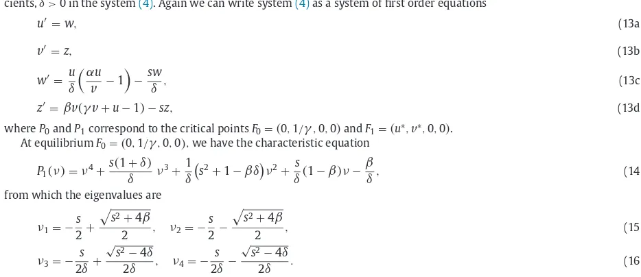
3if speedsc1=Fig. 1. Qualitative graphs of the characteristic polynomial withδ=0 and varyingsfor (a)P1(λ) in(9), and (b)P2(λ) in(12).
JE1=
⎛
⎜
⎝
1
s −α1s 0
0 0 1
αβ
αγ+1 αγαβγ+1 −s
⎞
⎟
⎠
. (11)It follows the characteristic equation of(11)atE1is
P2
(λ)
=λ
3+s2−1 s
λ
2−1+
αγ
αβγ
+1λ
+β
s. (12)
FromP2(
λ
), there is exactly one negative root and two positive roots or a pair of complex roots with positive real parts (see Fig. 1b). Thus there is a two dimensional unstable manifold based at equilibriumE1.2.2. Predator and prey diffuse,
δ
>0Generally, predator and prey move at different rates. In a case where both of the species move, one could be moving a little faster than the other or both of them are moving at a similar rate. For example, equal diffusivity of both species (
δ
=1) is due to spatial mixing from turbulence in a lake or in the sea. For such a case, one can assume that the magnitude of the diffusivity for the predator (zooplankton) and the prey (phytoplankton) is the same[22].For general species, let’s assume that the predator and prey diffuse at different rates. Then the ratio of the diffusion coeffi-cients,
δ
>0 in the system(4). Again we can write system(4)as a system of first order equationsu=w, (13a)
v
=z, (13b)w= u
δ
α
uv
−1−sw
δ
, (13c)z=
β
v
(γ
v
+u−1)
−sz, (13d)whereP0andP1correspond to the critical pointsF0=
(
0,1/γ
,0,0)
andF1=(
u∗,v
∗,0,0)
. At equilibriumF0=(
0,1/γ
,0,0)
,we have the characteristic equationP1
(ν)
=ν
4+s
(
1+δ)
δ
ν
3+1δ
s2+1−βδ
ν
2+δ (
s 1−β)ν
−β
δ
, (14)from which the eigenvalues are
ν
1= − s2+
s2+4
β
2 ,
ν
2= −s
2−
s2+4
β
2 , (15)
ν
3= − s2
δ
+√
s2−4
δ
2
δ
,ν
4= −s
2
δ
−√
s2−4
δ
2
δ
. (16)FromEq. (15), the eigenvalue
ν
1is always positive whileν
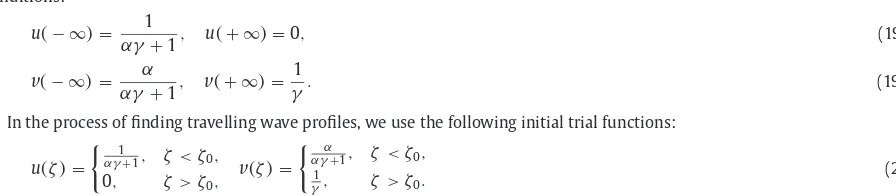
2is always negative. From(16), ifs≥2 √Fig. 2. Qualitative graphs of the characteristic polynomial withδ>0 and varyingsfor (a)P1(ν) in(14), and (b)P2(ν) in(18).
Fig. 2a). In our example, we use
δ
=2 to indicate predator’s diffusion rate is twice than the prey’s. There is a one dimensional unstable manifold and a two dimensional stable manifold based at equilibriumF0. For 0<s<2√
δ
,the trivial equilibriumF0is a spiral point on the stable manifold. Therefore, if the travelling wave solution exists, the possible minimum speed of system(13) for biologically relevant solution with non-negativeuandv
iss≥2√
δ
. (17)Withssatisfying condition(17), a realistic solution may exist which tends tou=0 and
v
=1/γ
asζ
→ +∞. At the non-trivial equilibriumF1=(
u∗,v
∗,0,0)
,we have the following characteristic equation:P2
(ν)
=ν
4+s
(
1+δ)
δ
ν
3+1δ
s2−1−
αβγ δ
αγ
+1ν
2−sδ
1+
αγ
αβγ
+1ν
+β
δ
. (18)FromP2(
ν
), there is exactly two negative roots or a pair of complex roots with negative real parts and two positive roots or a pair of complex roots with positive real parts (seeFig. 2b). Thus there is a two dimensional unstable manifold based at equilibriumF1.3. Numerical results
In this section, we describe how we solve a two-point boundary value problem given by system(4)and we simulate the full PDE problem(3)for both
δ
=0 andδ
=2.3.1. Travelling wave profiles
We use a relaxation or collocation method[23]to solve the travelling wave system(4)together with the following boundary conditions:
u
(
− ∞)
= 1αγ
+1, u(
+ ∞)
=0, (19a)v
(
− ∞)
=α
αγ
+1,v
(
+ ∞)
= 1γ
. (19b)In the process of finding travelling wave profiles, we use the following initial trial functions:
u
(ζ)
= 1αγ+1,
ζ
<ζ
0,0,
ζ
>ζ
0,v
(ζ)
= ααγ+1,
ζ
<ζ
0, 1γ,
ζ
>ζ
0.(20)
30 40 50 60 70 0
0.2 0.4 0.6 0.8 1
u, v
s increasing
s increasing
[image:6.544.168.378.57.225.2]predator,u prey,v
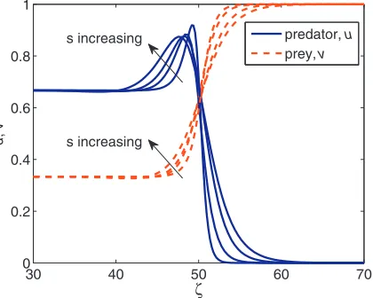
Fig. 3.Numerical solution of the travelling wave system(5)obtained from relaxation method withα=0.5,β=0.9,γ=1,δ=0,ζ0=50,with various speeds s=0.5,1,1.5,2.
and in contrast prey numbers decrease due the predation activity. After passing the interaction regime, both predator and prey stabilise at the coexistence equilibrium.Fig. 3also shows the solution of the system(5)with various wave speeds. As we found in(10),scan be any value greater than zero. Assincreases, we observe that the peak in predatoruis slightly decreasing.
In system(5), each parameter
α
,β
,γ
has different effects to the properties of the travelling wave solution. Different values ofα
andγ
affect the location of the coexistence equilibrium(
1/(αγ
+1)
,α
/(αγ
+1))
and the predator extinction equilibrium (0, 1/γ
), respectively. The variableβ
does not have any significant impact to the travelling wave of the preyv
,but the density of the predatoru, decreases asβ
increases. This is the result of the predator’s carrying capacity is dependent on the availability of the prey. Thus, any slight change in the system will affect the numbers of the predators. Also, this behaviour is caused by the nature of the system(5)whereβ
is written as the factor for the growth terms inEq. (5b).For the case where both species diffuse (
δ
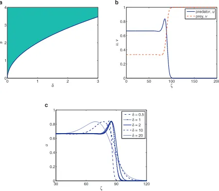
>0), we plot the region where the travelling wave of system(4)is possible from the speed condition(17).Fig. 4a shows the minimum speed curves=2√δ
=s∗that divides the parameter space into two regions. The shaded region represents parameter space wheres≥s∗and the unshaded region representss<s∗. We set the ratio of diffusion coefficients,δ
=2,which represents the diffusion parametersd1andd2in the dimensional system(2)and other parameters remain the same as before for all our travelling wave profiles. Withδ
=2,the minimum wave speed iss∗=2√2. Using this set of parameters (in the shaded region), we plot the travelling wave profile as shown inFig. 4b. However, if we plot the wave profile using parameter set in the unshaded region, we will have negative population density which is not biologically sensible thus it is not shown here.Fig. 4c shows the predator’s profile with different values of diffusivity parameter,δ
. The character of the travelling wave remains the same, but the region of solution expands asδ
increases due to the numerical computations to relax the solution at the left and right boundaries.3.2. Simulations
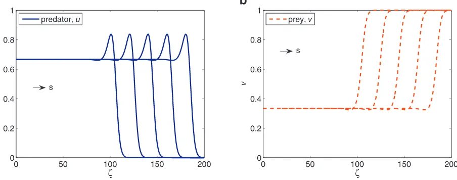
We numerically simulate the PDE system(3)via method of lines[30]with the initial conditions obtained from the relaxation method for
δ
=0 with fixed speeds=2 are shown inFig. 5. The distribution of each species is shown across the domain for time intervals of size 100 and we discretise one dimensional space into equal size ofn=2000 in a finite interval [0, 200]. In all simulations, we use Neumann boundary condition∂
u/∂
n=∂
v
/∂
n=0,which reflects no population can escape across the boundary.Fig. 5shows that the fixed wave profile moving to the right with constant speeds. We can observe that both equilibria are connected by the travelling wave solution – similar results as the relaxation method found in the previous section. The presence of predator at the right boundary induces the prey to increase and move. Once the predator starts consuming the prey, the prey numbers are reduced. The prey are depicted by a tanh-shaped kink solution whereas the predator shows a one-hump travelling wave as a result of consumption. Both predator and prey coexist at the left boundary. The behaviour of the travelling wave solution can be viewed similar relative to a dispersion of a soliton. Solitons are known to originate from the nonlinearity effects in the governing equations and have been shown to have a single hump-shaped that moves along thex-axis direction. In our case, the peak in the predator and a slight dip in the prey are induced by the nonlinear interaction terms found in system(5).
We also plot the solutions for
δ
=2 with minimum speeds∗=2√2 inFig. 6. Compared to the stationary caseδ
=0 inFig. 5, the waves travel further for the case withδ
=2. This shift is driven due to the effect of the diffusion parameterδ
. The greater value ofδ
, the further the populations move over space. In this case, the predator moves twice as fast compared to the prey.Fig. 4. (a) The curves=2√δ=s∗separates the shaded and the unshaded regions in the (s,δ) parameter space. Shaded region represents parameter space wheres≥2√δ,and the unshaded region represents parameter spaces<2√δ. (b) Wave profile of system(4)obtained from a relaxation method withα=
0.5,β=0.9,γ=1,δ=2,ζ0=100,ands=s∗=2
√
2. (c)uprofile with different values of diffusivity parameter,δ.
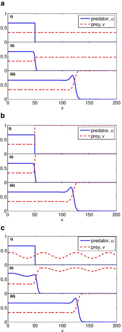
et al.[20]study a predator–prey system that depends on the choice of initial conditions. They found that for some small pertur-bation in an otherwise homogeneous distribution gives rise to a heterogeneous spatial distribution of species. However, they did not discuss travelling wave solution for the PDE problem. Dunbar[8]found travelling wave solution in a predator–prey system using a particular step-function form of initial conditions.
In our study, we simulate the PDE system(3)with several initial conditions: constant-gradient, step-function, and sinusoidal function. For all simulations, we solve(3)with a Neumann boundary condition and
δ
=2. The minimum wave speed according to the condition(17)is s∗=2√δ
=2√2.We begin with a simple step function for predatoruand constant distribution for prey
v
u
(
x,τ)
= 1αγ+1, x<x0,
0, x>x0,
v
(
x,τ)
=α
αγ
+1, (IC1)and then consider step functions for both species
u
(
x,τ)
= 1αγ+1, x<x0,
0, x>x0,
v
(
x,τ)
= ααγ+1, x<x0, 1
γ, x>x0,
(IC2)
and finally investigate a sinusoidal distribution in prey
v
u
(
x,τ)
= 1αγ+1, x<x0,
0, x>x0,
v
(
x,τ)
=α
αγ
+1+Asin2
π(
x−xo)
SFig. 5. Solutions of system(3)via method of lines with the initial conditions obtained from the relaxation method. Solutions are plotted on the same axes at
τ=5.7,12.7,19.6,26.7,33.7,40.7. Parameters areα=0.5,β=0.9,γ=1,δ=0 and fixed speeds=2.
Fig. 6. Solutions of system(3)via method of lines with the initial conditions obtained from the relaxation method. Solutions are plotted on the same axes at
τ=5.7,12.7,19.7,26.7,33.7. Parameters areα=0.5,β=0.9,γ=1,δ=2 and minimum speeds∗=2√2.
whereAandSare constants withA<αγα+1.
The simulations of the travelling waves with different initial conditions are given inFig. 7. For all three types of initial condi-tions, after some initial transients (seeFig. 7a (ii), b(ii), and c(ii)), the travelling wave profiles are similar to those found by the relaxation method inSection 3.1. These simulations show that a wide range of initial conditions for the PDE system will relax to a travelling wave. Hence, it demonstrates that the travelling wave solutions found in our work are attractors in the PDE system and are nonlinearly stable.
4. Conclusions
We have studied a spatio-temporal reaction-diffusion system modelling Leslie–Gower predator–prey population with dif-fusion. We showed that system(4)gives rise to a travelling wave solution that connects one critical point to the other. Using stability analysis, a minimum wave speed condition was derived for the case with diffusion parameter
δ
>0. The relaxation method is used to find the travelling wave profile for both casesδ
=0 andδ
>0. [image:8.544.47.499.281.459.2]predator and prey is robust to either how the two species initially encounter one another or external shocks to the population numbers.
Acknowledgements
HMS is grateful toUniversiti Tun Hussein Onn Malaysiaand the School of Physical, Environmental and Mathematical Sciences, UNSWCanberra for financial support.
References
[1] M.A. Aziz-Alaoui, Study of a Leslie–Gower–type tritrophic population model, Chaos Solitons Fractals 14 (2002) 1275–1293.
[2] A.A. Berryman, The origins and evolution of predator–prey theory, Ecology 73 (5) (1992) 1530–1535.
[3] F. Chen, L. Chen, X. Xie, On a Leslie–Gower predator–prey model incorporating a prey refuge, Nonlinear Anal.: Real World Appl. 10 (2009) 2905–2908.
[4] L. Chen, F. Chen, Global stability of a Leslie–Gower predator–prey model with feedback controls, Appl. Math. Lett. 22 (2009) 1330–1334.
[5] J.B. Collings, The effects of the functional response on the bifurcation behavior of a mite predator–prey interaction model, J. Math. Biol. 36 (1997) 149–168.
[6] Y. Du, S.B. Hsu, A diffusive predator–prey model in heterogeneous environment, J. Differ. Equ. 203 (2004) 331–364.
[7] Y. Du, R. Peng, M. Wang, Effect of protection zone in the diffusive leslie predator–prey model, J. Differ. Equ. 246 (2009) 3932–3956.
[8] S.R. Dunbar, Travelling wave solutions of diffusive Lotka–Volterra equations, J. Math. Biol. 17 (1983) 11–32.
[9] M.E. Gilpin, M.L. Rosenzweig, Enriched predator–prey systems: theoretical stability, Science 177 (4052) (1972) 902–904.
[10] G.W. Harrison, Comparing predator–prey models to Luckinbill’s experiment with didinium and paramecium, Ecology 76 (2) (1995) 357–374.
[11]Y. Huang, P. Weng, Traveling waves for a diffusive predator–prey system with general functional response, Nonlinear Anal.: Real World Appl. 14 (2013) 940–959.
[12] W. Ko, K. Ryu, Non-constant positive steady-state of a diffusive predator–prey system in homogeneous environment, J. Math. Anal. Appl. 327 (2007) 539– 549.
[13] A. Korobeinikov, A Lyapunov function for Leslie–Gower predator–prey models, Appl. Math. Lett. 14 (2001) 697–699.
[14] A. Korobeinikov, Stability of ecosystem: global properties of a general predator–prey model, Math. Med. Biol. 26 (2009) 309–321.
[15] A. Korobeinikov, W.T. Lee, Global asymptotic properties for a Leslie–Gower food chain model, Math. Biosci. Eng. 6 (3) (2009) 585–590.
[16] Y. Kuang, E. Beretta, Global qualitative analysis of a ratio-dependent predator–prey system, J. Math. Biol. 36 (1998) 389–406.
[17]P.H. Leslie, A stochastic model for studying the properties of certain biological systems by numerical methods, Biometrika 45 (1/2) (1958) 16–31.
[18] P.H. Leslie, J.C. Gower, The properties of a stochastic model for the predator–prey type of interaction between two species, Biometrika 47 (3/4) (1960) 219–234.
[19] C. Li, G. Zhang, Existence and non-existence of steady states to a cross-diffusion system arising in a Leslie predator–prey model, Math. Methods Appl. Sci. 35 (2012) 758–768.
[20]A.B. Medvinsky, S.V. Petrovskii, I.A. Tikhonova, H. Malchow, B.L. Li, Spatiotemporal complexity of plankton and fish dynamics, SIAM Rev. 44 (2002) 311–370.
[21]V. Naudot, E. Noonburg, Predator–prey systems with a general non-monotonic functional response, Physica D 253 (2013) 1–11.
[22]S.V. Petrovskii, B.L. Li, Models of interacting populations, Exactly Solvable Models of Biological Invasion, Chapman & Hall/CRC Press, Boca Raton, 2006.
[23]A. Quarteroni, A. Valli, Numerical Approximation of Partial Differential Equations, Springer Science & Business, Heidelberg, 2009.
[24]S.E. Riechert, Spiders as representative ‘sit-and-wait’ predators, Natural Enemies: The Population Biology of Predators, Parasites and Diseases, John Wiley & Sons, 2009.
[25]S. Rinaldi, S. Muratori, Y. Kuznetsov, Multiple attractors, catastrophes and chaos in seasonally perturbed predator–prey communities, Bull. Math. Biol. 55 (1) (1993) 15–35.
[26]S. Ruan, D. Xiao, Global analysis in a predator–prey system with non-monotonic functional response, SIAM J. Appl. Math. 61 (4) (2000) 1445–1472.
[27]H.M. Safuan, H.S. Sidhu, Z. Jovanoski, I.N. Towers, Impacts of biotic resource enrichment on a predator–prey population, Bull. Math. Biol. 75 (10) (2013) 1798–1812.
[28]H.M. Safuan, H.S. Sidhu, Z. Jovanoski, I.N. Towers, A two-species predator–prey model in an environment enriched by a biotic resource, Anziam J. (2014).in press.
[29]H.M. Safuan, I.N. Towers, Z. Jovanoski, H.S. Sidhu, Coupled logistic carrying capacity model, Anziam J. 53 (2012) C172–C184.
[30]W.E. Schiesser, The numerical method of lines, Integration of Partial Differential Equations, Academic Press, San Diego, 1991.