An optimized algorithm for simultaneous routing and buffer insertion in multi terminal nets

www.arpnjournals.com

AN OPTIMIZED ALGORITHM FOR SIMULTANEOUS ROUTING AND

BUFFER INSERTION IN MULTI-TERMINAL NETS

C. Uttraphan1, N. Shaikh-Husin2

1

Embedded Computing System (EmbCoS) Research Focus Group, Department of Computer Engineering, Faculty of Electrical and Electronic Engineering, Universiti Tun Hussein Onn Malaysia, Batu Pahat, 86400,

Malaysia

2_{Universiti Teknologi Malaysia, Johor Bahru, 81310, Malaysia}

E-Mail: [email protected], [email protected]

ABSTRACT

In today’s VLSI design, one of the most critical performance metric is the interconnect delay. As design dimension shrinks, the interconnect delay becomes the dominant factor for overall signal delay. Buffer insertion is proven to be an effective technique to minimize the interconnect delay. In conventional buffer insertion algorithms, the buffers are inserted on the fixed routing paths. However, in a modern design, there are macro blocks that prohibit any buffer insertion in their area. Many conventional buffer insertion algorithms do not consider these obstacles. This paper presents an algorithm for simultaneous routing and buffer insertion using look-ahead optimization technique. Simulation results show that the proposed algorithm can produce up to 47% better solution compared to the conventional algorithms. Although research has shown that simultaneous routing and buffer insertion is NP-complete, however, with the aid of look-ahead technique, the runtime of the algorithm can be reduced significantly.

Keywords: Buffer insertion, VLSI routing, VLSI design automation, dynamic programming.

INTRODUCTION

Interconnect is a wiring system that propagates signals to the various functional blocks in VLSI circuits. When VLSI technology is scaled down, gate delay and interconnect delay change in opposite directions. Smaller devices lead to less gate switching delay. In contrast, thinner wire increases wire resistance and signal propagation delay. As a result, interconnect delay has become the dominating factor for VLSI circuit performance (ITRS 2013; Alpert et al. 2009). Among the available techniques, buffer insertion has been proven to be one of the best techniques to reduce the interconnect delay for a long wire. The main challenge in interconnect buffer insertion is how to determine the optimal number of buffers and their placement in the given interconnect tree. The most influential and systematic technique was proposed by van Ginneken (van Ginneken 1990). Given the possible buffer locations, this algorithm can find the optimum buffering solution for the fixed signal routing tree that will maximize timing slack at the source according to Elmore delay model (Elmore 1948).

Recently, many techniques to speed-up van Ginneken algorithm and its extensions were proposed, such as in (Shi and Li 2003; Shi and Li 2005; Li and Shi 2006b; Li and Shi 2006a; Li et al. 2012). However, van Ginneken algorithm and its extensions can only operate on a fixed routing tree. They will give optimal solution when the best routing tree is given, but produce a poor solution when a poor routing tree is provided, especially when there are obstacles in the design. In today’s VLSI design, some regions may be occupied by predesigned libraries such as IP blocks and memory arrays. Some of these regions do not allow buffer or wire to pass through and some regions only allow wire to go through but are restricted for any buffer insertion. Therefore, buffer insertion has to be performed with consideration of this buffer and wire obstacles (Alpert

et al. 2009; Khalil-Hani and Shaikh-Husin 2009). The best way to handle the obstacles is to perform the routing and buffer insertion simultaneously using a grid graph technique. However, research has shown that simultaneous routing and buffer insertion is NP-complete (Hu et al. 2009). The available known techniques today are either using dynamic programming to compute optimal solution in the worst-case exponential time or design efficient heuristic without performance guarantee.

The dynamic programming algorithm such as RMP (Recursive Merging and Pruning) algorithm can find an optimal buffering solution for multi-terminal nets (Cong and Yuan 2000), but it is not efficient when the number of sinks and the number of possible buffer locations are big as the search space is very large. Indeed, Hu et al. show that the searching in RMP is NP-complete. They also proposed a heuristic algorithm to solve multi-terminal nets buffer insertion problem by constructing a performance driven Steiner tree where an alternative Steiner node is created if the original Steiner node is inside the obstacle area (Hu et al. 2003). The algorithm is called RIATA for Repeater Insertion with Adaptive Tree Adjustment. RIATA is very fast because it operates on a fixed tree. However, the quality of the solution may not be good enough if many paths of the adjusted tree still overlap with the buffer obstacles.

solve the simultaneous routing and buffer insertion for single-sink net problems.

This paper is organized as follows: section 2 gives problem formulation, section 3 provides the background of the study, section 4 describes the proposed algorithm, section 5 presents the experimental results and section 6 summarizes the conclusion.

PROBLEM FORMULATION

The simultaneous routing and buffer insertion problem in VLSI layout design is essentially a buffered routing path search problem. In this work, it is formulated as a shortest-path problem in a weighted graph specified as follows. Given a routing grid graph G = (V, E) corresponding to VLSI layout where v∈V and e∈E is a set of internal vertices and a set of internal edges respectively, with a source vertex S0∈V, n sink vertices s1, s2, …, sn∈V, n – 1 Steiner vertices m1, m2, …, mn-1∈V, a

buffer library B and a wire parameter W. The goal is to find a routing path simultaneously with buffer insertion such that the delay at the source is minimized. A vertex vi ∈V may belong to the set of buffer obstacle vertices, denoted VOB or a set of wire obstacle vertices, denoted as VOW. A buffer library B contains different types of buffer. For each edge e

= u→v, signal travels from u to v, where u is the upstream vertex and v is the downstream vertex and u, v ∉ VoW. A uniform grid graph illustrating some of the parameters for the problem formulation is shown in Figure 1.

Figure 1: A uniform grid graph G = (V, E)

BACKGROUND

In simultaneous routing and buffer insertion algorithm, the VLSI layout is represented by a uniform 2D grid graph as shown in Figure 1. Each wire segment (each edge of the graph e∈E) is modelled as π-model RC circuit as shown in Figure 2a while the buffer model is shown in Figure 2b. The label cw and rw are the capacitance and resistance per wire segment respectively while rb, cb and db

are the output resistance, input capacitance and intrinsic delay of the buffer respectively.

(a) (b)

Figure 2: (a) Wire segment model (b) Buffer model

The goal of the algorithm is to determine the best location of buffers on a given interconnect (at the vertex between each segment) in order to optimize the Elmore delay. The delay is calculated for each segment starting from a sink vertex toward the source (this is called upstream computation). The computation is characterized by two parameters, which are downstream capacitance and downstream delay. Each capacitance-delay (c, t) pair is called a candidate solution. This candidate solution is expanded toward the source by the following operations (these operations are also known as path expansions): (1) Wire expansion: Expand the candidate solution from vertex v to u by inserting a wire segment between v and u as shown in Figure 3. If (c, t) is the candidate solution at vertex

v, then the new candidate solution at vertex u is (c’, t’) pair given by

w c c

c′= + and 

    

+ +

=

′ t r c c

t _w w

2 . (1)

Figure 3: Wire expansion from vertex v to vertex u for upstream path expansion

(2) Wire expansion terminated by buffer: Expand the candidate solution from vertex v to u by inserting a wire segment between v and u and insert the buffer at vertex v as shown in Figure 4. If (c, t) is the candidate solution at vertex

v, then the new candidate solution (c’, t’) at vertex u is given by

b

w c

c

c'= + andt rw cw cb+db+rbc+t

   

 ₊

= 2

' . (2)

Figure 4: Wire expansion from vertex v to vertex u and buffer insertion at v

(3) Branch merging: If the solution reach a Steiner vertex, the candidate solution from the left branch (c, t)left is merged

with the candidate solution from the right branch (c, t)right.

The merging solution (c’, t’) is given by

left right c

c

c'= + and t'=max

(

)

.

s source t cR

t = + (4)

PROPOSED ALGORITHM

Design Descriptions of the Proposed Algorithm

HRTB-LA algorithm comprises of five main stages as shown in Figure 5. The first stage is the graph construction phase where the 2D grid graph is constructed to represent the VLSI layout.

Figure 5: Main stages in HRTB-LA

The tree modification is performed in stage two. The tree adjustment in HRTB-LA is adopted from (Hu et al. 2003) where the initial tree is adjusted according to the obstacles before the path expansions are performed. According to (Hu et al. 2003), the difficulty of buffer obstacle problem occurs when a Steiner vertex lies in an obstacle region, which eliminates opportunities for buffer insertion at the vertex. The key idea of tree adjustment is to consider an alternative Steiner vertex outside of the obstacle without changing the original topology.

The graph pruning in stage three is used to reduce the search space of the algorithm. The idea is to remove the redundant vertices from the graph before the search for path expansion is performed. Stage 4 is the look-ahead weight vector calculation, and stage 5 is the path expansion stage. The maze search starts from each sink towards the Steiner vertex where the branch merging operations are performed to create a new solution set. These solutions will be propagated toward the source and the best solution is selected as a final solution. As they are the most critical parts of the proposed algorithm, stages four and five of the algorithm are explained in more detail in the following sub-sections.

Look-ahead scheme

The look-ahead concept is a mechanism to reduce the search space of possible paths. The first idea was introduced in the field of artificial intelligence (Lin 1965; Newell and Ernst 1965). The idea is to limit the set of possible paths by using information of the remaining sub-paths toward the destination. The look-ahead concept was then adopted in the QoS routing in (Mieghem and Kuipers

2004) where the look-ahead was proposed to further limit the set of possible sub-paths when solving the MCP (multi-constraint paths) problem. In VLSI routing and buffer insertion problem, it was utilized by (Khalil-Hani and Shaikh-Husin 2009) but it was only for two-terminal nets. In this work, we extend this idea into the multi-terminal nets optimization. The concept of look-ahead is to maintain the lowest weight component wi∀ 1 ≤ i ≤ m from the source vertex to the destination vertex. This information provides each vertex u with attainable lower bound of wi(Pu→vdes) where vdes is the destination vertex. We denote by LA(u)the lower bound weight vector for vertex u, known as the look-ahead weight vector.

In HRTB-LA, the look-ahead weight vectors are used to guide the path expansion from one node to another node, i.e. from sink node to Steiner node and so on. These weights will be combined with the weights from normal path expansion to form a so-called predicted end-to-end delay. The look-ahead weight vectors are the resistance-delay (r, t) pair from a node (we call this as a start node) to the next downstream node (end node). In other words, the look-ahead weight vectors are the candidate solutions for the downstream path expansions. Hence, the computation for look-ahead weight vectors are as follows;

(1) Look-ahead wire expansion: Expand the candidate solution from vertex u to v by inserting a wire segment between u and v as shown in Figure 6. If (r, t) is the candidate solution at vertex u, then the new candidate solution (r’, t’) at vertex v is given by

r r

r'= w+ and c t

r r

t w w+

     ₊ =

2

' . (5)

Figure 6: Wire expansion from vertex u to vertex v for downstream path expansion

(2) Look-ahead wire expansion terminated by buffer: Expand the candidate solution from vertex u to v by inserting a wire segment between u and v and insert the buffer at vertex v as shown in Figure 7.

Figure 7: Wire expansion from vertex u to vertex v and buffer insertion at v

b

r

r'= and t r cw cb rw cw cb+db+t

  



 ₊

+ + =

2 ) (

' . (6)

To understand the concept of look-ahead, we now explain the look-ahead scheme using the following example. Figure 8 shows an interconnect tree with two sinks.

Figure 8: A sample tree

The corresponding 2D grid graph for the area between sink1 and Steiner node is shown in Figure 9. In Figure 9, Steiner node and sink1 are located in vertices 39 and 14 respectively. Vertices 12, 13, 26 and 27 are wire obstacle vertices VOW while vertices 40 and 41 are buffer obstacle vertices VOB. The computations for this illustration are performed using the following parameters; Load capacitance CL = 0.022 pF, wire resistance rw = 37.5 Ω/segment, wire capacitance cw = 0.1026 pF/segment, buffer input capacitance cb = 0.022 pF, buffer output resistance rb = 104.2 Ω, buffer intrinsic delay db = 20 ps and the source output resistance Rs = 104.2 Ω.

Figure 9: A 2D grid graph representing a tree in Figure 8 between Steiner node and sink1

At first, HRTB-LA transforms the 2D grid graph into a 1D graph. The 1D graph vertices is based on the shortest topological distance between Steiner vertex (start node) and sink1 vertex (end node) ignoring buffer obstacles

VOB. For example, the shortest topological distance between Steiner vertex and sink1 of Figure 9 is five; therefore, the 1D graph to calculate the look-ahead weight vectors has six vertices as shown in Figure 10, where topological distance between vertex 1 and vertex 6 is five. The look-ahead weight vectors are then calculated for each vertex in the 1D graph. Recall that the look-ahead weight vectors are the downstream candidate solutions, hence, they are computed using Eq. (5) and (6).

Figure 10: 1D grid graph

The look-ahead weight vectors for the graph in Figure 9 are shown in Figure 11. In the 1D graph, vertex 6 corresponds to the sink1 vertex in the original 2D graph. Vertex 5 in 1D graph corresponds to all the vertices in the original 2D graph that are four grids away from the Steiner node (vertices 28 and 56) while vertex 3 in 1D graph corresponds to vertices two grids away from the Steiner node (vertices 41 and 54), and so on. The vertex that exceeds the topological start-to-end node distance will not have any look-ahead vector. A special value, WeightMax is assigned as the look-ahead weight for these vertices.

WeightMax is the minimum delay at the end node taking into account the load capacitance CL and is given by

(

)

minrC t r t

WeightMax= L+ ∀ . (7)

The look-ahead weights will be combined with the weights from normal path expansion to form a so-called predicted end-to-end delay. The expansion is now guided by using the predicted end-to-end delay instead of the normal path expansion delay. This will reduce the number of candidates significantly because the candidate that has a predicted end-to-end delay greater than a known end-end-to-end delay will not be expanded. For a vertex v, the predicted end-to-end delay is given by

v LA LA

v t r c

t lay

EndToEndDe = + + (8)

where tv and cv are the accumulated delay and capacitance to vertex v from sink node respectively while tLA and rLA are the look-ahead delay and resistance for vertex v (i.e. the accumulated delay and resistance from Steiner node to node

v) respectively.

Path expansion

Path expansion is the process of constructing the path from sink nodes toward the source node. In HRTB-LA, path expansion is implemented using priority queue. The pseudo-code for the path expansion in HRTB-LA is shown in Figure 12.

In Figure 9, the path expansion begins from sink1 where the first (c, t) pair is (0.022, 0). At the beginning node, the delay is used as the key in the priority queue (line 1), hence the initial key value in the priority queue is 0. The first EXRTACT_MIN (extract the minimum key value from the queue) will extract the candidate solution from sink node for the next path expansion as there is only one key value in the queue (lines 3 – 4). The algorithm will check if the extracted candidate is the candidate from the start node (in this case the Steiner node). The extracted candidate is not from the start node, therefore, lines 6 – 7 are skipped.

added into the queue by invoking the function

InsertCandidate. The function InsertCandidate is shown in

Figure 13. In this function, the (c’, t’) pair will be checked for domination in lines 2 – 8.

Figure 11: Association of look-ahead weight vectors to input grid graph

Function: Path_Expansion

Input: Graph, G = (V, E) Wire parameter W

Buffer library B = {buf1, buf2, …., bufz}

Buffer obstacle VOB = {b1, b2, …, bm}

Wire obstacle VOW = {w1, w2, …, wp}

Look-ahead vectors, WeightLA Output: Candidate solutions for each node 1: Q ← delay at beginning node

2: while Q ≠ Ø do

3: EXTRACT_MIN from Q 4: extract (c, t) from list 5: if (v = Start)

6: compute (c’, t’) at Start node 7: InsertCandidate( ); 8: else

9: for each e ∈ E

10: if (w = 1) // if wire is allowed 11: compute (c’, t’) using Eq. (1) 12: InsertCandidate( ); 13: if (b = 1) // if buffer is allowed 14: for each buf in B do

15: compute (c’, t’) using Eq. (2) 16: InsertCandidate( );

Figure 12. Pseudo-code for the path expansion in HRTB-LA

In HRTB-LA, the candidate solution (c1, t1) is said to be

dominated by (c2, t2) if c1 > c2 and t1 > t2. The predicted

end-to-end delay is computed in lines 9 – 11 and it is pushed into the queue in line 12.

So far, the queue contains only the key associated with the candidate solution for vertex 28. The next EXTRACT_MIN will extract this candidate for the next path expansion. The expansion is from vertex 28 to vertex 42 only because vertex 27 is located in the wire obstacle. There are two types of expansion which are wire expansion (lines 10 – 12 in Figure 12) and wire expansion terminated by buffer (lines 13 – 16) because buffer insertion is allowed

at vertex 28. The path expansion is repeated until the first solution reaches the Steiner node (vertex 39).

Function: InsertCandidate

Input: Downstream capacitance c’ Downstream delay t’

Output: Predicted end-to-end delay in Q 1: for (i = 1; i <= TotalCandidateAt_v; i++)

2: if (c’ <= c[i] & t ’<= t[i]) //check for domination 3: remove (c[i], t[i]) from list;

//if new candidate dominates old candidate 4: insert (c’, t’) into list;

5: else if (c’ >= c[i] & t ’>= t[i])

6: return; //if old candidate dominates new candidate 7: else //if no domination

8: insert (c’, t’) into list; 9: for (j = 1; j <= LA_vectorAt_v; j++) 10: EndToEndDelay = tv + tLA[j] + rLA[j]cv;

11: Select minimum EndToEndDelay; 12: push EndToEndDelay into Q;

Figure 13: Pseudo-code for the insert candidate in HRTB-LA

In order to make look-ahead possible for a multi-terminal problem, a buffer must be inserted at the Steiner node such that end-to-end delay can be computed. By doing this, the quality of the solution may not be as good as the solution from the algorithm with normal path expansion (no look-ahead). However, from experimental results, the solution quality degradation is very small.

Time complexity of HRTB-LA

The proposed algorithm uses the Fibonacci heap data structure (Cormen et al. 2009) to implement the priority queue required for its operations. The advantage of Fibonacci heap over other heap algorithms such as binary heap and binomial heap is that it has much faster operations for the INSERT (used to add new key into the queue) and DECREASE_KEY (used to remove a redundant key from the queue) functions. These two functions are implicitly called in function InsertCandidate of LA. In HRTB-LA algorithm, the most time consuming part is the path expansion process. In the function Path_Expansion, the number of EXTRACT_MIN operations in the priority queue is upper bounded by the total number of vertices |V|. Since Fibonacci heap is used to implement the priority queue, therefore the amortized time for EXTRACT_MIN operation takes O(|B||V|2 log |V|) because the number of candidate solutions at each vertex is at most |B||V| (Zhou et al. 2000). In Fibonacci heap, each of the INSERT and DECREASE_KEY operations in the queue takes O(1). Hence, a wire expansion (lines 10 – 12 in Path_Expansion) takes O(|B||V|) times because the pruning and the end-to-end delay prediction operations are linear. Note that, the edge connection operation is bounded by O(|E|) where |E| is the total number of edges. Therefore the total computation time for wire expansions is O(|B||V||E|). Meanwhile, the second expansion (wire expansion terminated by buffer, in lines 13 – 16) takes O(|B|2|V||E|). Therefore the total running time for HRTB-LA algorithm is O(|M|(|B||V|2 log |V| + |B||V||E| + |B|2|V||E|)) ≈O(|M|(|B||V|2 log |V| + |B||V|2|E|)) where |M| is the total number of sinks and Steiner nodes. In practice, the number of |E| and |V| are small due to look-ahead scheme and graph pruning. This is proved by the experimental results presented in the following section.

RESULTS AND DISCUSSION

The proposed algorithm is implemented in C running on a 2.4 GHz Intel Core i5 PC with 4 GB RAM. Two set of experiments were performed. The first experiment was performed to prove that the solution quality of HRTB-LA (which applies the simultaneous routing and buffer insertion on adjusted tree) is better than algorithms which insert buffers on fixed routing tree. The second experiment was performed to demonstrate the effectiveness of the look-ahead scheme over the algorithm that performs normal path expansion (no look-ahead). We refer the algorithm with normal path expansion as HRTB (Uttraphan and Shaikh-Husin 2013) for Hybrid Routing Tree and Buffer insertion.

Experiment 1

In this test, the solutions from HRTB-LA were compared with the solutions from FBI (fast buffer insertion) algorithm (Li et al. 2012) and RIATA (Hu et al. 2003). The code for FBI algorithm is available for download at http://dropzone.tamu.edu/~zhuoli/GSRC/fast_buffer_inserti on.html. However, the code for RIATA is not available for download. Therefore, we coded our version of RIATA based on the descriptions in (Alpert et al. 2009) and (Hu et al. 2003). HRTB-LA, FBI and RIATA were tested on 21 different nets and graphs. The number of sink nodes ranges

from 3 to 9 sinks. Graph sizes are from 30 × 30 to 80 × 50 and the wire and buffer obstacles were randomly generated.

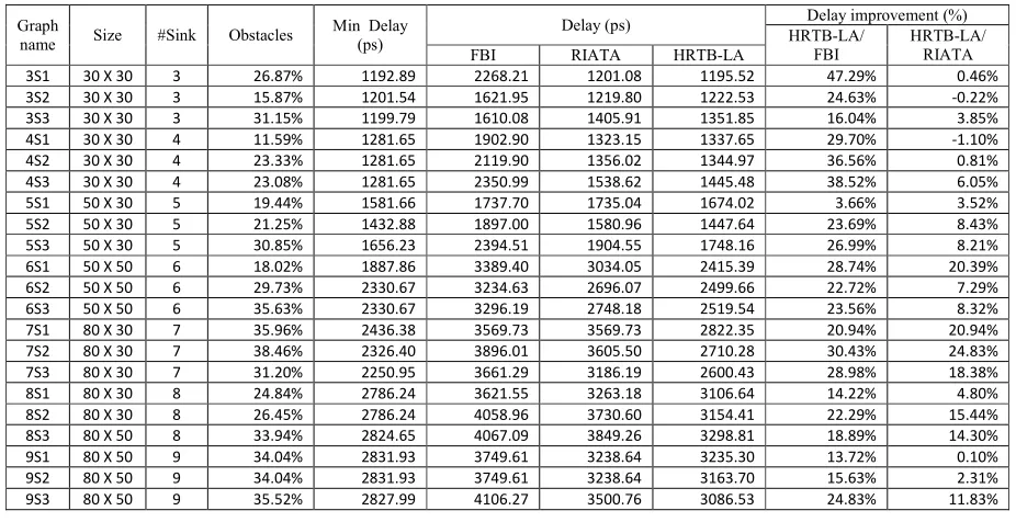
The test results are tabulated in Table 1. The table is organized as follows; columns 1 to 4 are the net name, graph size, the number of sink nodes in the net and the size of obstacle areas (wire/buffer) as compared to the size of the graph respectively. The fifth column shows the minimum delay after the net is optimized by FBI when there is no obstacle on the graph. This column indicates absolute minimum delay for the given net. These values are used as a reference in this test. Columns 6 to 8 are the delay at source obtained from FBI, RIATA and HRTB-LA algorithms respectively. Columns 9 and 10 are the delay improvement of HRTB_LA (in percentage) over FBI and RIATA respectively. As an example, for net 3S1, the graph size is a 30 × 30 grid (total vertices = 900). There are three sink nodes in this net and the obstacle areas are 26.9% of the graph. When the obstacles are ignored (can insert buffer anywhere on the net), the delay measured at source is 1192.89 ps. Meanwhile, when the obstacles are taken into account, the FBI algorithm returns delay at the source of 2268.21 ps. RIATA returns 1201.08 ps and HRTB-LA returns 1195.52 ps. This means that the delay improvement of HRTB-LA over FBI and RIATA are 47.29% and 0.46% respectively.

Clearly in all test cases, the solutions of HRTB-LA are better than the solutions from FBI where the highest delay improvement was recorded at net 3S1 which is 47.29%. For the comparison with RIATA, HRTB-LA improves the delay for most of the nets where the highest delay improvement was recorded for net 7S2 at 24.83%. However, the delays obtained from HRTB-LA are a bit larger than the delays obtained from RIATA for nets 3S2 and 4S1. This is because the obstacle areas on these nets are relatively small. Hence, the routing paths of HRTB-LA and RIATA are the same. Recall that a buffer must be inserted at each Steiner node in HRTB-LA and causes HRTB_LA to return a slightly higher delay. However, the solution degradations are relatively small which are 0.22% and 1.1% for net 3S2 and 4S1 respectively. In fact, if the obstacle areas are large (more than 18%), the solutions from HRTB-LA are better than the solutions from RIATA.

Experiment 2

In the second test, the solution quality, runtime and the number of candidate solutions produced by FBI, RIATA, HRTB and HRTB-LA algorithms are compared. The algorithms are performed on a randomly generated net with 25 sinks. The size of the grid is 100 x 100 which is equivalent to 20 mm × 20 mm layout size. The wire and buffer obstacles are 20% and 10% of the graph respectively.

18485 ps and the runtime is 1.56 s. The delay at source obtained from HRTB and HRTB-LA are 18073 ps and 18120 ps respectively while the recorded runtime are 5.61 s and 5.38 s respectively. When there are two or more types

of buffer in the library (cases 2 - 6), the solution quality for all algorithms are improved.

Table 1: Delay at source comparison between FBI, RIATA and HRTB-LA

Graph

name Size #Sink Obstacles

Min Delay (ps)

Delay (ps) Delay improvement (%)

HRTB-LA/ FBI

HRTB-LA/ RIATA

FBI RIATA HRTB-LA

3S1 30 X 30 3 26.87% 1192.89 2268.21 1201.08 1195.52 47.29% 0.46%

3S2 30 X 30 3 15.87% 1201.54 1621.95 1219.80 1222.53 24.63% -0.22%

3S3 30 X 30 3 31.15% 1199.79 1610.08 1405.91 1351.85 16.04% 3.85%

4S1 30 X 30 4 11.59% 1281.65 1902.90 1323.15 1337.65 29.70% -1.10%

4S2 30 X 30 4 23.33% 1281.65 2119.90 1356.02 1344.97 36.56% 0.81%

4S3 30 X 30 4 23.08% 1281.65 2350.99 1538.62 1445.48 38.52% 6.05%

5S1 50 X 30 5 19.44% 1581.66 1737.70 1735.04 1674.02 3.66% 3.52%

5S2 50 X 30 5 21.25% 1432.88 1897.00 1580.96 1447.64 23.69% 8.43%

5S3 50 X 30 5 30.85% 1656.23 2394.51 1904.55 1748.16 26.99% 8.21%

6S1 50 X 50 6 18.02% 1887.86 3389.40 3034.05 2415.39 28.74% 20.39%

6S2 50 X 50 6 29.73% 2330.67 3234.63 2696.07 2499.66 22.72% 7.29%

6S3 50 X 50 6 35.63% 2330.67 3296.19 2748.18 2519.54 23.56% 8.32%

7S1 80 X 30 7 35.96% 2436.38 3569.73 3569.73 2822.35 20.94% 20.94%

7S2 80 X 30 7 38.46% 2326.40 3896.01 3605.50 2710.28 30.43% 24.83%

7S3 80 X 30 7 31.20% 2250.95 3661.29 3186.19 2600.43 28.98% 18.38%

8S1 80 X 30 8 24.84% 2786.24 3621.55 3263.18 3106.64 14.22% 4.80%

8S2 80 X 30 8 26.45% 2786.24 4058.96 3730.60 3154.41 22.29% 15.44%

8S3 80 X 50 8 33.94% 2824.65 4067.09 3849.26 3298.81 18.89% 14.30%

9S1 80 X 50 9 34.04% 2831.93 3749.61 3238.64 3235.30 13.72% 0.10%

9S2 80 X 50 9 34.04% 2831.93 3749.61 3238.64 3163.70 15.63% 2.31%

9S3 80 X 50 9 35.52% 2827.99 4106.27 3500.76 3086.53 24.83% 11.83%

Table 2: Solutions quality, runtime and number of candidate solutions for Experiment 2

Buf

FBI RIATA HRTB HRTB-LA

delay (ps)

Runtime (s)

# Candidate

delay (ps)

Runtime (s)

# Candidate

delay (ps)

Runtime (s)

# Candidate

delay (ps)

Runtime (s)

# Candidate

1 18854 0.37 - 18485 1.56 6480 18073 5.61 12725 18120 5.38 1985

2 18774 0.39 - 18381 1.71 11318 17955 6.29 22316 17983 5.32 3985

3 18724 0.43 - 18307 2.06 17471 17904 9.16 34651 17924 5.39 7259

4 18713 0.53 - 18289 2.8 23525 17891 14.6 46811 17912 5.52 9869

5 18707 0.72 - 18277 4.09 29426 17880 25.1 58636 17909 5.71 12589

6 18707 0.92 - 18277 5.68 35260 17880 40.37 70240 17909 6.07 14984

(b)

(c)

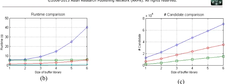
Figure 14: Plot of test results (a) delay (b) runtime (c) number of candidate solutions

Figure 14 is the plot of the performance comparisons from Table 2. All the performance metrics are plotted against the size of the buffer library. For delay comparison in all test cases, clearly HRTB and HRTB-LA outperformed RIATA and FBI because HRTB and HRTB-LA found the best path for each node by utilizing the simultaneous routing and buffer insertion (maze search). As expected, the solution quality of HRTB is slightly better than HRTB-LA but only a small degradation is observed (less than 1%). Again, this is due to buffer insertion requirement at merging nodes for HRTB-LA to facilitate look-ahead scheme. In terms of runtime, HRTB seems to have an exponential relationship with the number of buffers in the library as the number of candidate solutions grow quickly because of the maze search in the path expansions. The runtime of FBI is the fastest, followed by the runtime of RIATA. This is because FBI and RIATA only perform one direction path expansion. Although HRTB-LA also uses maze search like HRTB, its runtime is linear and comparable to FBI and RIATA. The number of candidate solutions also proves that HRTB-LA is very efficient. In fact, the number of candidate solutions from HRTB-LA is lower than the number of candidate solutions from RIATA. For HRTB-LA, the depth first search in look-ahead scheme allows the algorithm to find the destination as quickly as possible and eliminates unnecessary path expansions later on.

CONCLUSION

In this paper, the hybrid of the simultaneous and post routing approach for multi-terminal nets is described. By utilizing a given routing path, the proposed algorithm, HRTB-LA adjusts the routing tree if the Steiner node lies in the buffer obstacle. The rerouting process, simultaneously with buffer insertion are performed later on. The results show that the proposed algorithm can produce a better solution compared to other algorithms. To speed up the runtime of the algorithm, the novel look-ahead which were proven to be successful in optimizing the two-terminal nets (Khalil-Hani and Shaikh-Husin 2009) are adopted in this work. Presented results demonstrate the advantage of the path expansion with the aid of look-ahead compared to the normal path expansion. The time complexity of HRTB-LA is O(|M|(|B||V|2 log |V| + |B||V|2|E|)). Although the O -notation shows that the runtime of the algorithm can grow exponentially, however, we do not observe this phenomenon in experiment. This is because the number of

|E| and |V| are small due to graph pruning and look-ahead scheme.

ACKNOWLEDGEMENT

This work is supported by Higher Education Department, Ministry of Education Malaysia and Universiti Tun Hussein Onn Malaysia (UTHM). The author would like to thank Zhuo Li et al. for providing the FBI code.

REFERENCES

Alpert, C.J., Mehta, D.P. and Sapatnekar, S.S. (2009).

Handbook of algorithms for physical design automation, Auerbach Publications.

Cong, J. and Yuan, X. (2000). Routing tree construction under fixed buffer locations. In Proc. 37th Annual Design Automation Conference. ACM, pp. 379–384.

Cormen, T.H., Leiserson, C.E. and Rivest, R.L. (2009).

Introduction to Algorithms 3rd ed., Boston, MA: McGraw-Hill.

Elmore, W. (1948). The transient response of damped linear networks with particular regard to wideband amplifiers.

Journal of Applied Physics, 19(1), pp.55–63.

van Ginneken, L.P.P.P. (1990). Buffer placement in distributed RC-tree networks for minimal Elmore delay. In

Proc. Int. Symp. Circuits and Systems. Ieee, pp. 865–868.

Hu, J. et al. (2003). Buffer insertion with adaptive blockage avoidance. IEEE Trans. Computer-Aided Design of Integrated Circuits and Systems, 22(4), pp.492–498.

Hu, S., Li, Z. and Alpert, C.J. (2009). A fully polynomial time approximation scheme for timing driven minimum cost buffer insertion. In Proceedings of the 46th Annual Design Automation Conference DAC ’09. New York, New York, USA: ACM Press, pp. 424–429.

ITRS (2013). The international technology roadmap for semiconductors: Interconnect

Khalil-Hani, M. and Shaikh-Husin, N. (2009). An optimization algorithm based on grid-graphs for minimizing interconnect delay in VLSI layout design. Malaysian Journal of Computer Science, 22(1), pp.19–33.

on Design, Automation and Test in Europe. IEEE, pp. 484 – 489.

Li, Z. and Shi, W. (2006b). An O (mn) time algorithm for optimal buffer insertion of nets with m sinks. In Asia and South Pacific Conference on Design Automation. IEEE, pp. 320–325.

Li, Z., Zhou, Y. and Shi, W. (2012). An O (mn) time algorithm for optimal buffer insertion of nets with m sinks.

IEEE Trans. Computer-Aided Design of Integrated Circuits and Systems, 31(3), pp.437–441.

Lin, S. (1965). Computer Solutions of the Traveling Salesman Problem. Bell System Technology, 44(10), pp.2245–2269.

Mieghem, P. van and Kuipers, F. (2004). Concepts of exact QoS routing algorithms. IEEE Trans. Networking, 12(5), pp.851–864.

Newell, A. and Ernst, G. (1965). Search for generality. In

IFIP congress. pp. 17–24.

Shi, W. and Li, Z. (2005). A fast algorithm for optimal buffer insertion. IEEE Trans. Computer-Aided Design of Integrated Circuits and Systems, 24(6), pp.879–891.

Shi, W. and Li, Z. (2003). An O(nlogn) time algorithm for optimal buffer insertion. Design Automation Conference, IEEE, pp.580–585.

Uttraphan, C. and Shaikh-Husin, N. (2013). Hybrid Routing Tree with Buffer Insertion under Obstacle Constraints. In

IEEE Student Conference on Research and Development.