Induction motor modelling using fuzzy logic

INDUCTION MOTOR MODELLING USING FUZZY LOGIC

MOHD NASRI BIN HASHIM

A project report submitted in partial fulfillment of the requirement for the award of the Master of Electrical Engineering

Faculty of Electrical and Electronic Engineering Universiti Tun Hussein Onn Malaysian

ABSTRACT

Fuzzy logic has been widely used in many engineering applications since this can overcome the limitations of conventional method of data analysis, modelling and system identification, and control system. The capability of dealing with highly non-linear system modelling that is so complex that require absolute analytical design make these mathematical model architecture more popular in the engineering field. This project is addressed on the modelling of induction motor Auto-Regressive with exogenous input (ARX) model structure using fuzzy logic. In this case fuzzy logic is combined with neural network of said Neuro Fuzzy (ANFIS) is applied and has functioned as estimator of the ARX model parameters. The ARX model of induction motor is estimated from its input output data. Input variable is voltage and output variable is speed. The experimental results show that the best model responses have similarly trend with the motor actual responses, final prediction error is 0.00873, loss function is 0.00807, and fit to working data is 67.22%. It means the model produce from system identification able adopt the motor dynamic and can use for replacing real motor for analysis and control design.

vi

ABSTRAK

TABLE OF CONTENTS

DECLARATION OF THESIS STATUS EXAMINER’S DECLARATION

TITLE i

STUDENT’S DECLARATION ii

DEDICATION iii

ACKNOWLEDGEMENTS iv

ABSTRACT v

ABSTRAK vi

TABLE OF CONTENTS vii

LIST OF TABLES ix

LIST OF FIGURES x

LIST OF SYMBOLS AND ABBREVIATIONS xi

CHAPTER 1 INTRODUCTION 1

1.1 Project Background 1

1.2 Problem Statements 3

1.3 Project Objectives 3

1.4 Scopes of the project 3

CHAPTER 2 LITERATURE REVIEW 5

2.1 Introduction 5

2.2 Induction Motor Basics 5

2.2.1 The Stator 6

2.2.2 The Rotor 8

2.2.3 Torque Production 9

viii

of an Induction Motor 10

2.4 System Identification 13

2.5 Linear model structures 15

2.6 Nonlinear model structures 19

2.7 Parameter estimation 20

2.7.1 Linear regression – linear least squares 20

2.8 Nonlinear methods 22

2.9 Types of models 23

2.10 ARX models 26

CHAPTER 3 METHODOLOGY 28

3.1 Background 28

3.2 Project Flowchart 28

3.2.1 Start 29

3.2.2 Literature Review 29

3.2.3 Simulation 29

3.3 Identification Procedure 31

3.3.1 Experimental design and data collection 33 3.3.2 Raw data pre-processing 34 3.3.3 Model structure determination 34

3.3.4 Estimation 34

3.3.5 Validation 34

CHAPTER 4 RESULT AND ANALYSIS 35

4.1 ARX Model Identification 36 4.2 ANFIS Model for System Identification 37

CHAPTER 5 DISCUSSION AND CONCLUSION 44

5.1 Discussion 44

5.2 Conclusion 44

5.2 Recommendation for further development 45

REFERENCES 46

APPENDIX1 48

APPENDIX2 52

LIST OF TABLES

x

LIST OF FIGURES

2.1 Inside view of an induction motor 6 2.2 Resultant flux vectors as a sum of the

three phase currents at 90 and 180 7 2.3 Air-gap flux density of a 3-phase,

2-pole, two-layer induction motor winding 7

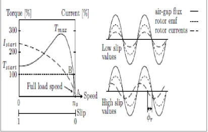
2.4 Torque speed relationship 9

2.5 A set of inputs u is fed to the process and model. Output y is disturbed by noise v, denotes the model

output and e the error difference yˆ 15

2.6 RC Circuit 24

2.7 Black Box Identification 25

3.1 Methodology Flowchart 30 3.2 The identification procedure 33 4.1 Data Collection of Induction Motor 35 4.2 Training Data and ARX Prediction 36 4.3 Checking Data and ARX Prediction 37 4.4 Training and Checking Error 41

4.5 Estimate the Model 42

LIST OF SYMBOLS AND ABBREVIATIONS

ARX Autoregressive Model with Exogenous input

AR AutoRegressive

MA Moving average

X eXogeneousinputs

NARX Nonlinear Autoregressive Model with Exogenous in

IM Induction Motor

Ψ Resultant flux vectors

emf Electromotive force

V Voltage

Im Magnetizing current

s Synchronous speed

n Speed of the rotor

ns Speed of the magnetic field mmf Magnetomotive force

r Current lag by a angle r Motor speed

Ls and Lr Stator and rotor self-inductance

s Stator supply angular frequency

e Noise

y The matrix of observed outputs of a system

Ɵ The system model parameters

CHAPTER 1

INTRODUCTION

1.1 Project Background

The induction motor, which is the most widely used motor type in the industry, has been favoured because of its good self-starting capability, simple and rugged structure, low cost and reliability. Along with variable frequency AC inverters, induction motors are used in many adjustable speed applications which do not require fast dynamic response. The concept of vector control has opened up a new possibility that induction motors can be controlled to achieve dynamic performance as good as brushless DC motors.

In order to understand and analyze vector control, the dynamic model of the induction motor is necessary. It has been found that the dynamic model equations developed on a rotating reference frame is easier to describe the characteristics of induction motors. Any method for speed prediction is based on a model of the motor and the drive. The best accuracy of prediction for an induction motor is needed. Today, there are many choices of modelling techniques. One of them is system identification where it identifies the behaviour of a given system by estimating the model from input and output data. The estimated model is useful to simulate and predict the behaviour of the system. Not limited to that, the fitted model can be employed to regulate the output of plant.

Exogenous Input where its autoregressive variable comprising of past output data and the exogenous input variable is represented as past input data (Bjorn Sohlberg, 2005). In other word, this model is used to estimate the parameters in the model structure from historical input-output data of a scrutiny system.

The ARX model is among the simple Models for linear process and it is easy to be implemented (Xiangdong Wang et all, 2008). This project is addressed the modelling of induction motor based on the ARX model structure using fuzzy logic. Fuzzy models become useful when a system cannot be defined in precise mathematical terms. The non-fuzzy or traditional representations require a well structured model and well defined model parameters. Even if the structure is known, numerical model representations usually become irrelevant and computationally inefficient as the complexity increases. Moreover, there may be a lot of uncertainties, unpredictable dynamics and other unknown phenomena that cannot be mathematically modelled at all. Therefore, when a system cannot be modelled with traditional methods for the reasons stated above, then fuzzy logic offers an efficient mathematical tool in handling many practical problems. The main contribution of fuzzy control theory is its ability to handle many practical problems that cannot be adequately handled by conventional control methods.

3 mathematical way of defining a fuzzy model of a nonlinear system without necessitating any human knowledge.

1.2 Problem Statements

System identification in control theory is about building a mathematical model, which identifies any dynamical system or signal, based on observed inputs and outputs data. The key problem in modelling induction motor is to find a suitable model structure. To avoid this problem, in this project nonlinear ARX modelling has been chosen as a candidate model of induction motor and fuzzy logic as an estimator algorithm.

1.3 Project Objectives

The objectives of this project consist of the following: 1. To design fuzzy logic for system modelling.

2. To derive ARX model structure for induction motor candidate model. 3. To collect input output data of induction motor through experimental

test.

4. To identify mathematical model of induction motor using fuzzy logic. Algorithm based on induction motor input output data.

5. To validate the identified induction motor mathematical model.

1.4 Scopes of the project

The scopes of the project are:

3. ARX model of induction motor is identified applying fuzzy logic 4. Identified model is validated with noise test and several prediction

methods.

CHAPTER 2

LITERATURE REVIEW

2.1 Introduction

Mathematical modelling is of fundamental importance in science and engineering. It is very useful and presents a compact way of summarizing the knowledge about a process or system. This need for identifying and modelling the observation data appears in a wide range of applications. The process of model building consists of mapping the relationship between observed data from the system, onto a mathematical structure. Mathematical models can be constructed based on either known results from physics or data analysis.

2.2 Induction Motor Basics

iron. The rotor slots are also skewed to reduce non-linear effect such as harmonics and torque pulsation.

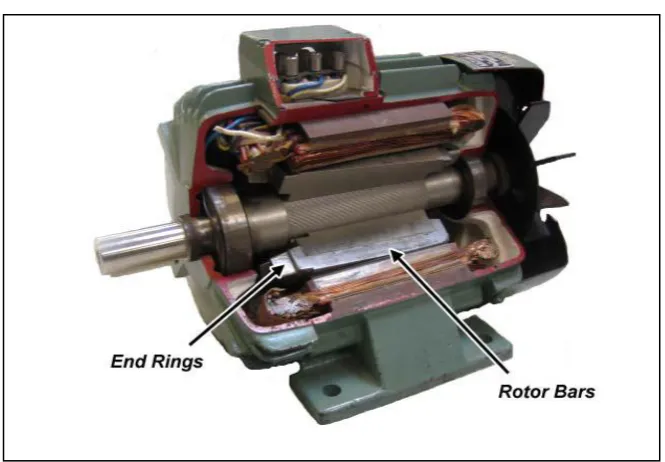
Figure 2.1: Inside view of an induction motor

2.2.1 The Stator

7

Figure 2.2 Resultant flux vectors as a sum of the three phase currents at 90 and 180

Since every stator conductor is cut by the rotating magnetic field an alternating electromotive force (emf) E will be induced opposing the voltage V according to Lenz’s law. The stator can thus be described by the equation V = ImR + E, which shows the relation between the applied voltage V ,the magnetizing current Im (example the current that sets up the flux) and the induced (emf) E. If the flux decreases, so will the emf. This makes the magnetizing current increase which in turn makes the flux increase and hence the emf. The magnetizing current will adjust itself so that the emf always equals the applied voltage.

2.2.2 The Rotor

Torque producing currents are induced in the rotor bars by interaction with the air-gap flux wave, the rotor is dragged along by the rotating field. If the rotor is held stationary there will be a high current induced in the rotor bars since the wave will cut the bars at a high velocity. If, on the other hand, the rotor is rotating with the same velocity as the magnetic field, there will be no current induced in the rotor bars. The slip is defined as the relative velocity between the speed of the magnetic field (ns), which is also known as the synchronous speed, and the speed of the rotor (n).

(2.1)

9

2.2.3 Torque Production

With a small slip, the frequency of the induced emf in the rotor is low which makes the reactance of the rotor low (in this case the rotor is predominantly resistive) and thus the rotor current in phase with the rotor emf which in turn is in phase with the air-gap flux. As a result the torque-speed relationship for small slip is approximately a straight line. As the slip increases, both the rotor emf and frequency increases. With increased frequency the rotor inductive reactance also increases which makes the current lag by a angle rshown in the right part of Figure 2.4.

2.3 Mathematical Dynamic Model of an Induction Motor

The induction motor can be represented in the stator stationary reference frame (- coordinate axes) by a second order differential equation relating the stator input voltages and currents as:

h vs

dt dv h i g dt di g dt i d 0 s 1 s 0 s 1 2 s 2   

 (2.2)

Where the coefficients of equation (2.2) are given in the following way

                    r r s r o s r r r s s r o r s s r r s j T L h L h j T R L g j L R L R g        1 1 1 1 (2.3)

These coefficients are functions of the machine parameters and motor speed (r).Where Ls and Lr are stator and rotor self inductance respectively, and are defined by Ls = Lm + Lls and Lr = Lm + Llr , Tr = Lr/Rr is a rotor time constant and

11



 s

s

s v  jv

v (2.4)

  s s ji i   s

i (2.5)

Where vs_,vs_ are the -axis and -axis stator voltage components in the stationary

reference frame and i_s,i_s are the corresponding currents. Using equations (2.2)-(2.4), the second derivative of the stator current, components at constant speed can be derived as

                                                                 _                       5 4 3 2 1 2 2 2 2 A A A A A i i v v dt dv dt di i i v v dt dv dt di dt di dt i d dt di dt i d s r s s s r s s s r s s s r s s s r s s r s                       (2.6) Where s s r s r s r s s r r

s R R

A R A L A L R L R A        

 _{2 3 4}

1 , , , and A

L R_{r s}

s

5  

Applying the following constraints to equation (2.6), Constraint 1: v_s  V_s cos_st

Constraint 2: v_s V_s sin_st

Constraint 4: is_  Is sin(st)

Where s is the stator supply angular frequency (rad./sec.) and  is the phase angle between the stator voltage and current components. This results in the following equations:





    

 

 s s s ss r s r s

r s s

s A v Av A i A v A i

A

i _{2 3 1 2 5}

4 2

) (

1 _{   }

 

 (2.7)





 _{ } s s s ss r s r s

r s s

s Av A v A i A v A i

A

i _{3 2 1 2 5}

4 2 ) ( 1      

 (2.8)

Equations (2.7) and (2.8) represent the model of the induction motor. These equations may be put in the form

 

 



 s s s r s rs

s Kv K v Ki K v K i

i  ₁  ₂  ₃  ₄  ₅ (2.9)

 

 



 s s s r s r s

s K v Kv Ki K v K i

i  ₂  ₁  ₃  ₄  ₅ (2.10) Where





K A

A

s

s s r

1 2 2 4    

   (2.11)





K A

A

s s r

2 3 2 4   

   (2.12)





K A

A

s

s s r

3 1 2 4    

   (2.13)





K A

A

s s r

4 2 2 4    

   (2.14)





K A

A

s s r

5 5 2 4   

13 This is for constant known motor speed and if the leakage inductance in both stator and rotor circuits are considered the same (M. Liwschitz-Garik and C. C. Whipple,1961). (Lls  Llr), equations (2.11)-(2.15) may be solved together to obtain the electrical machine parameters in the form.

1 5 K K R s s 

 (2.16)

2 1 3 / K K R K

L s s

s

 

 (2.17)

1 2 2 K L K

R r s

r



 (2.18)

2 2 2 ) ( K R L K R r s r s s r

s _{  }



 

 (2.19)

L_m  L2_s 



2.4 System Identification

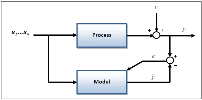
referred to simply as modelling (P. V. d. Bosch, 1994). System identification techniques are applied in, example the process industry to find reliable models for control design (Y. Zhu & T. Backx,1993). The input-output data is collected from experiments that are designed to make the data maximally informative on the system properties that are of interest. The model set specifies a set of candidate models in which the "best" model according to a well-defined criterion will be searched for. In prediction error methods, the sum of the square of prediction errors, example the mismatch between the real measured output and the model output is often used as a criterion (L. Ljung, 1987). Selecting the three entities, data, model set, and criterion are very important steps in an identification procedure. When the data is available, the model set is chosen, and a criterion is selected, the model in the model set that best fits the data according to the specified criterion has to be found. In general, a model set is parameterized and a parameter estimation algorithm is used to find the parameter values such that the model behaviour fits best to the data according to the criterion. Finally, model validation tests are performed.

15

Figure 2.5: A set of inputs u is fed to the process and model. Output y is disturbed by noise v, denotes the model output and e the error difference yˆ

2.5 Linear model structures

The choice of model structure is a central concept in identification – in this section the most well-known structures are briefly introduced. This framework of model structures is often referred to as black box structure (A. Procházka, 1998), which covers a general set of systems without particular attention to physical constraints. A further distinction is often made between parametric and nonparametric models (O. Nelles, 2001). Parametric models represent the system through a finite set of parameters, example in a difference equation, which allows parametric methods to be used in identification. Hence, the discussion will deal almost exclusively with parametric models, with the parameters assumed to be time-invariant. Furthermore, the models presented are considered in discrete time only due to implementation reasons.

the first category, the most general representation (assuming a SISO system) can be obtained by filtering the input u by a linear filter G and filtering the stochastic white-noise term e by a corresponding filter H. The filters can generally be split into a nominator and denominator part (where A represents a possible common denominator of G and H), hence giving the model;

(2.21)

Where is the backward shift operator, . The polynomials A,

B, C, F and D are thus of the form;

(2.22)

Equation (2.21) represents the basic model for a linear system from which all linear models can be derived (L. Ljung,1983). This basic model structure is, however, seldom used, as it has proven to be too abstract. Instead, it is often preferred to start with the simplest model which has a possibility of describing the system adequately.

The simplest models for linear systems originate from econometrics, where models were built for stochastic time series (O. Nelles, 2001). The common equations featured only white noise as input and included the autoregressive (AR);

(2.23)

The moving average (MA);

(2.24)

17

(2.25)

These models served as building blocks for the subsequent ARX model (autoregressive with exogenous inputs), which contains both an autoregressive and input part. The ARX model is often referred to as the “the mother of all dynamical model structures” (L. Ljung.1983), as it is the most commonly used equation to model linear systems, defined as;

(2.26)

The model conforms to the basic difference equation form;

(2.27)

which signifies that the white-noise error term e(k) enters the equation directly. The finite impulse response model (FIR) is a special case of the ARX model, which is better known from filtering theory. The model considers only feedback in the input signal;

(2.28)

The use of ARX in identification is justified in many ways, the main reason being that the parameters of the model are easy to estimate (the predictor of the

Correlated noise can be modelled as a moving average (2.24), which inserted into (2.26) gives the popular ARMAX form;

(2.29)

A second more realistic structure for the noise is provided by the output error (OE) model, which assumes that the noise enters late in the process without sharing denominator dynamics. The model takes the form;

(2.30)

Where the noise is the direct error between the model and the real output. However optimal identification of this model, as opposed to the ARX, requires the simulated outputs, which result in a nonlinear regression (O. Nelles, 2001),(L. Ljung, 1987)

Identification of ARMAX and OE model generally involves the use of approximate linear nonlinear optimization method.

An alternative representation for both SISO and MIMO models is provided by state-space models (IIASA’s 20th Anniversary, System Identification, 2009). State-space models have the following representation in discrete timel

+

(2.31)

19

(2.32)

The expression is substituted in (2.29), yielding the relation;

⇒ (2.33)

If the system is SISO, H(q) is a transfer function, whereas MIMO systems will convert into a matrix of transfer functions. Correspondingly, a model in input-output form can be transformed into various state-space representations, provided it is proper. For a more detailed discussion, refer to (O. Nelles, 2001).

2.6 Nonlinear model structures

The selection of a black-box model structure becomes a more difficult problem when

one is dealing with nonlinear systems, although the nomenclature follows that of the

linear models. A general model including all nonlinear and linear models can be

described as;

(2.34)

(2.35)

The dilemma of choosing the regressor set is discussed further in (J. Sjöberg, H. Hjalmarsson & L. Ljung. Neural Networks in System Identification, 1994), from which the following can be concluded, applying both to nonlinear and linear modelling: The regressor can be limited to inputs and no past outputs, if the response time of the system is finite, i.e., only inputs within a finite time frame t affect the output. This construction has the disadvantage of potentially requiring a large number of past inputs. By including past outputs in the regressor, the system can model an infinite and complex response even with a small number of regressors. On the downside, this construction is prone to instability and adds up possible output noise in the model.

2.7 Parameter estimation

When the data and an appropriate model structure have been identified, the following step marks the identification of the parameters. The goal is to estimate the parameters in a way that provides an optimal fit of the model to the data. The majority of the traditional estimation techniques are based on the least-square estimate, which provides a standard method for solving linear regression problems. When the model parameters are constant, a linear estimation can be carried out batch, in a single step. Unfortunately, most real-world engineering problems are intuitively described by nonlinear functions, which require nonlinear optimization methods and a numerical “step-by-step” estimation process.

2.7.1 Linear regression – linear least squares

Linear regression is a common term for approaches where a line or a curve is fit to a set of observations, consisting of one or more independent variables and a (linearly) dependent variable (M. Verhaegen & V. Verdult, 2007). Assuming the dependence is described by a simple model.

21 The regression would imply estimating a and b over the observation set (in this case consisting of the independent variable X and dependent variable Y). In identification, a linear regression arises when the error between the estimated and real output is

described by a linear relationship (O. Nelles, 2001). This is a feature of the ARXmodels,

which can be proven by transforming the ARX model (2.26) into regression form;

(2.37)

Where, is a regression vector and contains the model parameters. If the noise e(k) is assumed white, the scalar product defines the best possible predictor for the output. Notably, the prediction error;

(2.38)

is now of the same form as the equation error e(k). The error for each prediction is hence linearly dependent on the parameter vector – exactly as the linear regression requires. The least-squares method is the most well-known way of solving any linear regression (M. Verhaegen & V. Verdult, 2007)(L. Ljung, 1987). Other identification

methods for linear regression exist, but are omitted from description here since they are

of larger interest in the statistics community. The least-squares method attempts to

minimize a squared loss function, in this case the squared sum of residuals;

(2.39)

This function can be minimized analytically by setting its derivative (gradient) to zero. The solution for a multi-parameter system is most conveniently obtained by transforming (2.39) into matrix form. This is done by defining a regression matrix, a vector of outputs y, and applying matrix algebra to obtain;

The gradient is given as a vector of partial derivatives of 

(2.41)

and the least-square estimates are determined by setting to zero, which yields the normal equation;

(2.42)

The least squares estimate is finally computed by inverting example with

Gaussian elimination, yielding;

= (2.43)

The least-squares method can also be used for estimation of certain nonlinear problems, providing the nonlinear function is linearly dependent on the parameters (G. D. Nicolao. System Identification: Problems and Perspectives, 1997). If the measurement samples involve varying degrees of uncertainty or relevance for the estimation, a variant known as weighted least squares can be used. Each measurement is weighted with a factor wk, which results in the modified final estimate;

(2.44)

Containing a diagonal matrix W with the elements wk

2.8 Nonlinear methods

23

(2.45)

Whereas linear least squares estimation is straightforward, nonlinear problems lack a corresponding one-step solution. Instead of estimating the parameters directly, the nonlinear methods approximate the function f locally, in a step-by-step process. An initial estimate is provided for the parameters, followed by iterative update through successive approximation, until a satisfying solution is obtained. Nonlinear parameter estimation is generally carried out by nonlinear optimization methods, which are not limited to solving equations of the least-squares form.

2.9 Types of models

To describe a process or a system we need a model of system. This is nothing new, since we use models daily, without paying this any thoughts. For example, when we drive a car and approaching a road bump, we slow down because we fell intuitively that when this speed is too high we will hit the head in the roof. So from experiences we have developed a model of car driving. We have a feeling of how the car will behave when reach the bump and how we will be affected. Here the model of situation can be considered as a mental model. We can also describe the model by linguistic terms. For example if we drive the car faster than 110km/h then we will hit the head at the roof. This is linguistic model, since the model uses words to describe what happens (Bjorn Sohlberg, 2005). A third way of describing the systems is to use

scientific relations to make a mathematical model , which describes in what way output signals respond due to changes in input signal. There are different types of models to represent the system.

For example a model of electrical network using Kirchhoff’s laws and similar theorems;

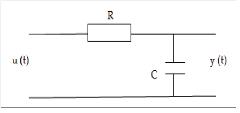
Figure 2.6 RC Circuit

In above RC-circuit where the relation between the input signal u(t) and output signal y(t) is given by Ohm’s law. The resulting model would be a linear differential equation with the unknown parameter M=RC, which can be estimated form an experiment with the circuit or formal nominal values of the resistor and the capacitor. A mathematical model is given by;

M.y(t) + y(t) = u(t) (2.46)

Similarly other processes can be modelled using scientific relations.

46

REFERENCES

A.Procházka. Signal analysis and prediction. Birkhäuser, 1998

Bjorn Sohlberg (2005). Book: Applied Modelling & Identification, Dalarna University, Sweden

C.T. Sun, “Rule-base structure identification in an adaptive-network based inference system,” IEEE Trans. On Systems, vol. 2, no. 1, pp. 64-73, 1994.

C. J. Park, I-K Jeong, H-K Kim and K. Wohn. Sensor Fusion for Motion Capture System Based on System Identification. Computer Animation 2000, pp.71, 2000.

D. W. Novotny and T. A. Lipo, “Vector Control and Dynamics of AC Drivers,” [Book}, Clarendon press. OXFORD, 1996

D. C. Karnopp, D. L. Margolis, and R. C. Rosenberg, System Dynamics: A Unified Approach. Wiley & Sons, 1990

G. Chen, T.T. Pham, J.J. Weiss, “modeling of control systems,” IEEE Trans. On Aerospace And Electronic Systems, vol. 31, no. 1, pp. 414-428, 1995

G.C. Mouzouris, J.M. Mendel, “Dynamic non-singleton logic systems for nonlinear modeling,” IEEE Trans. On Systems, vol. 5, no. 2, pp. 199-208, 1997.

G. D. Nicolao. System Identification: Problems and Perspectives. 12th Workshop on Qualitative Reasoning, June 1997

I. Eksin, C.T. Ayday, “identification of nonlinear systems,” International Conference On Industrial Electronics, Control And Instrumentation, vol. 2/3, pp. 289-293, 1993.

J. Sjöberg, H. Hjalmarsson and L. Ljung. Neural Networks in System Identification. 10th IFAC symposium on SYSID, pp. 49-71, 1994

L. Ljung. System Identification: Theory for the User. Prentice-Hall, 1987

M. Liwschitz-Garik and C. C. Whipple, “Alternating-Current Machines,” Van Nostrand., 1961

M. Nørgaard, O. Ravn, N. K. Poulsen and L. K. Hansen. Neural Networks For Modelling And Control Of Dynamic Systems: A Practitioner's Handbook. Springer, 2000

M. Verhaegen and V. Verdult. Filtering and System Identification: a Least Squares Approach. Cambridge, 2007

O. Nelles. Nonlinear System Identification. Springer, 2001

P. V. d. Bosch, Modelling, identification and simulation of dynamical systems.CRC Press Inc., 1994

System Identification. Paper Presented on IIASA’s 20th Anniversary. 20.9.2009 T. Kohonen. Self-Organizing Maps. Springer, 1995

T. Takagi, M. Sugeno, “identification of systems and its applications to modeling and control”, IEEE Trans. On Man and Cybernetics, vol. smc-15, no. 1, pp. 116-132, 1985

Xiangdong Wang, Ming Wei, Jianwen Zhao and Xiang Chen, Parameter Identification Based on SystemIdentification Toolbox in Matlab, Journal of Ordnance Engineering College. 2008, 20(4): 75-78