Forecasting Currency Exchange Rates via Feedforward
Backpropagation Neural Network
Joseph C. Chen*, Naga Hrushikesh R Narala
Department of Industrial & Manufacturing Engineering & Technology, Bradley University, USA
Copyright©2017 by authors, all rights reserved. Authors agree that this article remains permanently open access under the terms of the Creative Commons Attribution License 4.0 International License
Abstract
The latest globalization trends resulted in increasingly interdependent economies of nations and multinational firms. This may leave companies operating internationally at the mercy of the volatility in currency exchange rates. Forecasting these exchange rates became very important in international trade and commerce, as it involves key decisions of foreign investment, forward contracts and expanding business to new horizons. This research paper describes a Feedforward Backpropagation Neural Network (FBNN) model and its application to currency exchange rate forecasting. A study of FBNN model is conducted for forecasting exchange rates between Indian rupee and US dollar, based on previous data of inflation, real interest rates, gross domestic product (GDP), current account balances, government budget balances and debts of both countries. The weights used in neural networks were optimized using gradient descent and backpropagation method. Models with different hidden neuron layers were developed by comparing the actual exchange rates with forecasted monthly exchange rates from January 2001 to December 2014. The most effective model was then used to simulate exchange rates for the year 2015. The FBNN model with ten neurons in the hidden layer has the least Mean average percentage error (MAPE) value of 1.32% and is considered to be most impressive model.Keywords
Exchange Rates Forecasting, Feedforward Backpropagation, Neural Networks, Mean Average Percentage Error1. Introduction
A currency exchange rate is essentially what its name implies: it is the rate at which one would need to exchange one’s currency for the currency of other country. For any investment that is crossing borders, the risk and returns are dependent on the exchange rates between countries. The fluctuations pose a significant risk and uncertainty to every
sector involved in business [1]. It may be for an investment or a trade or a business, having knowledge of exchange rate is important to minimize risks and maximize profits.
Exchange rates are dependent on various economic factors. Flow patterns for majority of these factors follow non-linearity. Artificial neural networks are a natural choice for a forecast involving non-linear trends. Landavazo and Fogell [2] suggest changing all weights in the network simultaneously to reduce network operation time.
Back propagation algorithms are trained by a learning rule published by Rumelhart, Hinton and Williams [3]. Backpropagation algorithm makes use of two distinct passes, a forward/ activation pass followed by a backward/ weight adjusting pass, to scan the training data. The first (forward) pass presents an input vector to the first layer of the network, which propagates through the network one layer at a time [4]. The second (backward) pass attempts to correct this error by adjusting neuron’s weights in proportion to the error it generates [4]. The purpose of this research is to develop a feed forward back propagation neural network model that can forecast exchange rates with minimum errors.
2. Literature Review
(HMM). Though these advances could generate acceptable results, the flow of currency value depending on new economic developments cannot be anticipated.
Relative PPP [8] method is based on the concept of the “Law of one price”. Clements and Lan [9] proposed an approach to forecast exchange rates using purchase power parity theory. This model uses big mac data as inputs and Monte Carlo simulation to estimate the outputs. Both methods are impressive in forecasting linear behavior, but they cannot accurately estimate exchange rates against economic factors which have high volatility. For accurate long term estimations, a model that can consider multiple sources as inputs is needed. Because of this reason, a behavior model is needed. Hauner, Lee and Hajime [10] discuss multiple factors and their possible effects on exchange rates. To handle multiple inputs, a neural network with back propagation algorithm is used. Though this method may prove to be complex in nature, it has the potential to predict the results more accurate than any previous models. Difana Meilana and Ivan Richardo [11] developed a similar model to forecasting exchange rates of Indonesian rupiah and US dollar by choosing the variables as inflation, real income and interest rates. Mean average percentage error (MAPE) value for best model is around 0.69%. The dependency of exchange rate on the input variables is not discussed in [11]. Moreover the generated model is not used for further simulations.
This research intends to provide a methodology that can be used for any future designing. Simulating an already generated model provides a brief insight into the way the forecasting results can be estimated.
3. Methodology
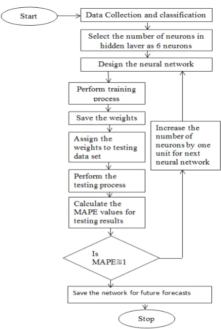
The objective of this paper is to cultivate a feed forward back propagation network having nominal number of hidden neurons. The first step is data collection and its classification. Output and input variables are defined in this phase. The collected data is then classified into training data and testing data. Then a regression analysis is conducted to find the dependency of input variables on output. The networks are trained with training data set to optimize their weights. Then the networks are tested with testing data set. The effectiveness of a network is measured by MAPE. The network with MAPE value closer to 1% is chosen for any future forecasting.
3.1. Data Collection and Classification
Exchange rates between two countries are depended on major factors such as differential inflation rates, real interest rates, gross domestic product (GDP), nation’s external debt, current account deficit and government budget deficit. The details of these factors [12, 13] are as follows:
Differential inflation rate is the difference between the countries inflation rate. It can be obtained only if
inflation rates of both countries are available for same time periods.
GDP of a country is the monetary value of all goods and services produced by it within a specific time period.
Current account balance of a nation directly reflects the country’s economic strength.
Real interest rates are the rate of interest one can receive after modifications from inflation. Data on real interest rates can be collected on an annual basis.
Government budget balance is the net amount balance to indicate spending of a nation’s government.
External debt of a country is the amount the country has borrowed from foreign banks, governments or institutions.
[image:2.595.313.552.310.543.2]
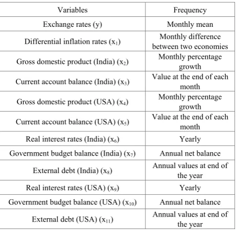
The output exchange rate y for Indian rupee against US dollar can be obtained by calculating the number of units of Indian rupee required to have one unit of US dollar.Table 1. Frequency of selected variables
Variables Frequency
Exchange rates (y) Monthly mean Differential inflation rates (x1) between two economiesMonthly difference
Gross domestic product (India) (x2) Monthly percentage growth
Current account balance (India) (x3) Value at the end of each month
Gross domestic product (USA) (x4) Monthly percentage growth
Current account balance (USA) (x5) Value at the end of each month
Real interest rates (India) (x6) Yearly
Government budget balance (India) (x7) Annual net balance
External debt (India) (x8) Annual values at end of the year
Real interest rates (USA) (x9) Yearly
Government budget balance (USA) (x10) Annual net balance
External debt (USA) (x11) Annual values at end of the year
Table 1 shows the frequency of selected variables. With the variables set, it is time to establish a time period over which reliable data can be collected. Though the economic data of US are available from 1970s, data for input variables on Indian economy are only available from 2001. So, the data is collected for a period of fifteen years from 2001 to 2015. Sources for obtaining these data are listed below: a The monthly monetary value of Indian rupee against
the US dollar and monthly GDP of two countries from January 2001 to December 2015 obtained from http://stats.oecd.org/
b The monthly inflation rates of both countries are collected from http://inflation.eu/
the number of input variables and 168 is the number of samples collected for 14 years (2001-2014). Apart from this input data, a 1 x 168 matrix with exchange rate values is created. 20 % of the input data is used for testing the output results. The remaining data is used for the purpose of training and validation, and is termed as training data set. The data for the year 2015 is used to simulate the output results from the developed Feedforward Backpropagation Neural Network (FBNN) model.
3.2. Regression Analysis on Dependency of Output on Input Variables
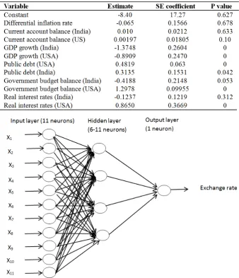
The analysis is conducted on MINITAB by using the training data sets. The results are shown in Table 2. The input variables together account for 91.1% of the variance (R2
adjusted = 0.911). The analysis of variance shows that the total data set has an F-statistic value of 152.70 and p value is zero. Even though some individual factors may not have any significant independent effect, the dataset altogether has a significant impact on the output (exchange rates).
3.3. Designing a Neural Network
[image:3.595.136.475.344.738.2]A neural network is defined by its training algorithm, learning function and output activation function. The performance function, number of hidden layers and number of neurons in the hidden layer have a significant effect on the level of performance of a neural network. This paper uses back propagation training algorithm with steepest gradient descent learning function. A log sigmoid function is considered as an activation function for the outputs. A performance function is helpful in adjusting the networks weights to improve performance. The number of hidden layer is generally considered to be one. The very first neural network is designed with six neurons (mean of number of input variables and the number of output variables) in the hidden layer, which is shown in Fig. 1. After verifying the results, if the performance of the network is not satisfactory, the no. of neurons is increased until the requirements are met [14, 15].
Table 2. Regression analysis on dependency of output on input variables
[image:3.595.136.477.345.741.2]Table 3. Parameter values at the start of the training process
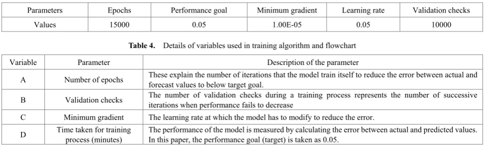
Parameters Epochs Performance goal Minimum gradient Learning rate Validation checks
[image:4.595.62.551.90.239.2]Values 15000 0.05 1.00E-05 0.05 10000
Table 4. Details of variables used in training algorithm and flowchart Variable Parameter Description of the parameter
A Number of epochs These explain the number of iterations that the model train itself to reduce the error between actual and forecast values to below target goal.
B Validation checks The number of validation checks during a training process represents the number of successive iterations when performance fails to decrease C Minimum gradient The learning rate at which the model has to modify to reduce the error.
D Time taken for training process (minutes) The performance of the model is measured by calculating the error between actual and predicted values. In this paper, the performance goal (target) is taken as 0.05.
3.4. Training a Neural Network
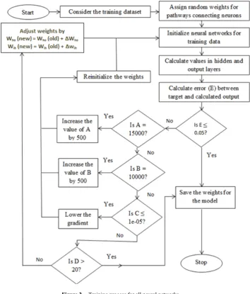
Parameter values at the start of the training process are shown in Table 3. Training process assists a neural network to adapt its weights in order to increase the performance of the network. The process is carried out until performance goal is achieved. Parameters including performance goal are specified before starting the process. Table 4 shows the details of variables used in training algorithm and flowchart. Fig 2 and Fig 3 are the training process for all neural networks and flowchart for testing process.
The algorithm for training process [11] is as follows: Step 1: Consider the training data set.
Step 2: Initialize all weights to small random values. Step 3: Initialize network with training data. Step 4: Calculate values in hidden and output layer. Step 5: Calculate error between target and calculated outputs.
Step 6: If error is close to zero, save the weights and stop or else go to step 7.
Step 7: If A is equal to 15000, increase the value of A by 500 and continue to step 10, or else go to step 8.
Step 8: If B is equal to 10000, increase the value of B by 500 and continue to step 10, or else go to step 9.
Step 9: If C is lower than 1e-05, lower the gradient and continue to step 10, or else go to step 11.
Step 10: Reinitialize the weights and go to step 3.
Step 11: If D is greater than 20, save the weights for the model and stop the training process.
Step 11: Correct the weights of line leading to output unit. Who (new) = Who (old) + ΔWho (1)
ΔWho = αδoOh,
Where Who is the weight connecting hidden layer to output
layer, α is the learning rate, Oh is the output at hidden layer,
δo is the error given by the following
δo = Oo (1-Oo)(To-Oo)
Step 12: Compute the weights of line leading to hidden unit.
Wih (new) = Wih (old) + Δwih (2)
Δwih = αδhOi
Where Wih is the weight connecting input layer to hidden
layer, α is the learning rate, Oi is the output at input layer, δh
is the error given by the following
δh = Oi(1-Oi) (ΔδoWho) (3)
Step 13: Update these weights in step 3 and repeat the process for each pattern in the training set
3.5. Testing a Neural Network
In the final stage, the saved weights from training process are assigned to the testing dataset. Testing algorithm for this process is as follows:
Step 1: Consider testing data set for testing process. Step 2: Assign the saved weights from training process. Step 3: Develop the hidden layer values from below equation
Xh = Xi Wih (i = 1,2,..k) (h = 1,2,…m) (4)
Step 4: Develop the output layer values from below equation
Xo = Xh Woh (h = 1,2,…m) (o = 1,2,…n) (5)
Step 5: Generate the output by sigmoid activation function f (x) = 1/ (1+ exp(-Xo)) (6)
Figure 2. Training process for all neural networks
Figure 3. Flowchart for testing process
The outputs generated by the networks test data are compared with target outputs. The accuracy of these models is MAPE and mean square error (MSE). MAPE approach is generally used to measure the accuracy of the forecasting method. Fig.4 is the flowchart summarizing the neural network development.
PE, MAPE and MSE values [11] are obtained from the equation 7, 8 &9 respectively.
PE = (𝑦𝑡−ŷ𝑡)
𝑦𝑡 x 100% (7)
MAPE =
∑
𝑛|𝑃𝐸𝑛|1 (8)
MSE = 1
n
∑
(yt− ŷt) 2 ni=1 (9)
where, n = number forecast, yt = actual value at t, ŷt =
[image:5.595.134.489.84.500.2] [image:5.595.106.251.517.738.2]Figure 4. Flowchart summarizing the neural network development If MAPE value is closer to 1%, the neural network can be considered for future research, or else, the number of neurons in the network is increased by one unit and the whole process is performed until satisfactory MAPE values are obtained. The neural network that can generate results with MAPE value closer to 1% is chosen to simulate the forecast
exchange rates for year 2015.
4. Results and Discussion
A total of six neural networks are created, trained and testing process is conducted on them. The end parameters of six networks are shown in Table 5. Although all the networks started with same parameters, detailed in Table 4, the conditions under which the training process terminated is different for every network.
Out of the six trained networks, network 3 and network 6 are the only networks that could not reach the performance goal. Network 3 could only attain performance goal of 0.112 during its training process that lasted 20 minutes. The training process of network 6 has to be stopped manually, as there was no improvement in performance beyond 0.496. The reason for this abnormality is because of minimum gradient. Even with a minimum gradient of 1e-013, the network terminated its training process. Table 6 shows the MAPE and MSE of the six trained networks. After training, the networks are tested by comparing the generated outputs with actual exchange rates.
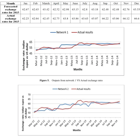
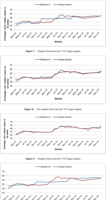
[image:6.595.60.288.81.421.2]The MAPE value, defined in Eq. (8) is used to measure the accuracy of neural models. Network 1 has a MAPE value between actual and forecast values as 3.723%. Similarly, the MAPE value, for network 5, is 1.32% which is the lowest among six networks. This concludes that network 5 has the best prediction accuracy within six models.
[image:6.595.80.530.551.661.2]Table 7 shows detail month by month prediction and actual currency exchange rates in year 2015 via network 5. Fig 5-10 show the outputs from each network vs. actual exchange rates and Fig. 11 shows actual results vs. forecasted results (year 2015) from an FBNN model with ten hidden neurons.
Table 6. Comparison of the performance of forecasted results
[image:7.595.78.524.211.650.2]Table 7. Forecasted values via network 5 comparing the actual exchange rates every month for year 2015
Figure 5. Outputs from network 1 VS Actual exchange rates
Figure 7. Outputs from network 3 VS Target outputs
Figure 8. Test outputs from network VS Target outputs
Figure 9. Outputs from network 5 VS Target outputs
[image:8.595.134.478.86.397.2]Figure 11. Actual results VS Forecasted results (year 2015) from an FBNN model with ten hidden neurons.
5. Conclusions
The designed feed forward backpropagation model forecasts exchange rates based on historical data of countries. Although all networks have generated acceptable [11] MAPE values, network 5, the model with ten neurons in hidden layer has generated the least MAPE value of 1.32%. Hence, network 5 is used for forecasting the values of year 2015. The results of the forecast are as follows:
The MAPE value for 12 month forecast is 2.481%.
From Fig 10, one can observe that the results are good for the first seven months (January to July).
The deviation for these months is less than 0.5.
For the last 5 months, the deviation of estimated results from actual results has taken a significant number.
Major contributors to MAPE value are the differences between actual and forecasted results from the last 5 months.
These fluctuations are in accordance with the volatility of global oil prices.
6. Recommendations
A crucial factor that the researcher ignored is the price of some commodities can have a direct impact on the strength of a countries currency. For US dollar, such commodity is oil and for Indian rupee, it is gold. According to Selien De Schryder and Gert Peersman [17], oil demand and the US dollar exchange rate are interdependent. So, based on the observation, the recommendations for future research are as follows:
Oil prices or oil demand and gold prices can be considered as input variables for future research.
Designing neural networks with different learning and performance function.
Updating the learning algorithm with improved evolutionary methods such as gene expression programming and simulated annealing.
Creating an online database that can store the current work and any future improvements.
REFERENCES
[1] Aaditya Mattoo, Prachi Mishra and Arvind Subramanian (March 2012) Spillover effects of Exchange Rates: A study of the Renminbi, International Monetary Fund.
[2] Landavazo, D.G., Fogell, G.B. (2002) Evolved neural networks for quantitative structure activity relationships of anti-HIV compounds, IEEE press, Piscataway, New Jersey. [3] Rumelhart, Hinton and Williams (1986) Learning internal
representations by back propagating errors, Nature, 323: 533-536.
[4] Raủl Rojas (2013) Neural Networks: A systematic introduction, Springer science & business media, 7: 152-174. [5] J.T. Yao, H.-L. Poh, T. Jasic (1996) Foreign exchange rates
forecasting with neural networks, in: Proceedings of the International Conference on Neural Information Processing, Hong Kong, pp. 754–759
[6] Philip, A. A., Taofiki, A. A., Bidemi, A. A. (2011). Artificial Neural Network Model for Forecasting Foreign Exchange Rate. World of Computer Science and Information Technology Journal (WCSIT), vol. 1, no. 3, pp. 110-118. [7] David E. Allen, Michael Mcaleer, Shelton Peiris and Abhay K.
Singh (2015) Nonlinear time series and neural network models of exchange rates between the US dollar and Major currencies. Tinbergen Institute discussion paper, 125-III.
[8] Jacob A. Frenkel (1983) Exchange rates and International Macroeconomics, 1-18, University of Chicago Press.
[9] Clements, K. W., and Y. Lan (2006). “A New Approach to Forecasting Exchange Rates.” Discussion Paper No. 06.29, Economics Program, The University of Western Australia. [10] David Hauner, Jaewoo Lee, and Hajime Takizawa (May 2010)
In Which Exchange Rate Models Do Forecasters Trust, International Monetary Fund (IMF).
[11] Difana Meilani and Ivan Richardo (2012) "Currency exchange rate forecasting using artificial neural networks backpropagation method", Int. J. Green Comput., vol. 3, issue 2: 14-33.
[12] James Stoker (1999) The Government Deficit and the Exchange rate, Review of International Economics, Vol. 7, issue 4: 753-763.
[14] W. Zou, Y. Li and A. Tang (2009) Effects of the number of hidden nodes used in a structured-based neural network on the reliability of image classification, Neutral Computing & Applications, vol. 18, no. 3, pp. 249-260.
[15] Saurabh Karsoliya (2012) Approximating number of hidden layer neurons in multiple hidden layer BPNN architecture, International Journal of Engineering Trends and Technology,
vol. 3-issue 6: 714-717.
[16] R.K.Bansal, A. Goel, Manoj K. Sharma (2009) MATLAB and its applications in engineering, Pearson education India, pp. 369-371.