Intelligent optimization algorithm and the application in mechanical design

Journal of Chemical and Pharmaceutical Research, 2014, 6(6):2830-2843

Research Article

_{CODEN(USA) : JCPRC5}

ISSN : 0975-7384

Intelligent optimization algorithm and the application in

mechanical design

Xia Jiansheng

*1,2

, Dou Sha Sha

1

, Yang Zirun

1

and Li Qingzhu

1

1

Yancheng Institute of Technology, Yancheng, China

2

Nanjing University of Aeronautics & Astronautics, Nanjin, China

ABSTRACT

Mechanical optimization design is a new design method in the development foundation of the modern mechanical design theory, the traditional design repeats the analysis of product performance passively and doesn’t design product parameters actively, which often cost too much money and manpower, and the application of optimization design in mechanical design can make the scheme achieve some optimization results in the design requirements specified, without consuming too much computational effort. Through the concrete examples, introduces the steps and method of setting up mathematical model of the mechanical optimization design. A brief overview of some optimization algorithm, such as genetic algorithm, artificial neural network, simulated annealing algorithm, Ant algorithm, tab search algorithm, particle swarm algorithm and hybrid algorithm combined some of them. The corresponding mathematical models of algorithm are established, according to the actual mechanical design problems, and used to solve the established mathematical model by computer, so as to obtains the optimal design scheme.

Key words: Mechanical design, Ant colony algorithm, Cellular ant algorithm

_____________________________________________________________________________________________

INTRODUCTION

With the development of production, economy and technology, optimization idea gradually was infiltrated in all human activities. When people are in rational behavior in a job; always want more efficiency as far as possible, try to find the best way to finish it, this is the optimization method. In other words, the purpose of optimization is to find the optimal method (the shortest time, the least human resources, material and equipment) to complete our work. In recent years, optimization technology is becoming more and more popular, and developed very well in many engineering fields, such as engineering design, resource allocation, production planning and scheduling, urban planning and so no. Engineer and management faces many optimization problems in practice, such as: how to select the parameters to not only meet the requirements but also reduce the cost in engineering design; how to meet the basic requirements of all aspects and obtain good economic benefit in resource allocation; how to raise GDP and profit in the production plan; how to arrange the school, shops, factories, hospitals, residential and other single bit reasonable layout in the city construction planning to be more convenient for people, more conducive to the city from all walks of life. These problems are optimization problems, which are to achieve the most reasonable and optimization solution[1][2].

operations research provided the optimization methods to solve the problem that classical calculus method and variation method cannot. Mathematical programming theory lays a theoretical foundation for the design optimization in 1950s. Computer and computing technologies provide powerful tools for optimization design in 1960s[3].

In recent years, some algorithms developed very rapidly and get good application effect, such us: genetic algorithm, Ant algorithm, simulated annealing and artificial neural network as the representative of the intelligent optimization algorithms[4].

Application of hybrid method of several algorithms used in scheme optimization and the parameter optimization of mechanical optimization design, it has important theoretical significance and application value of solving some mechanical optimization design has been more difficult issue[5].

EXPERIMENTAL SECTION

The model and implementation of ant algorithm

Ant algorithm initially originated from the thought of the network path，the one-dimensional case, which leads to

the solution of n-dimensional space function.

A typical constrained function optimization problem can be written as follows

)

(

max

Z

=

f

x







∈

−

≤

]

,

[

,

2

,

1

,

0

)

(

.

b

a

X

m

i

X

g

t

s

i

L

It does not consider the constraints are met or not in the search process, using the conventional penalty function method to meet it, converting all constraint equations into the objective function, and directly evaluating objective function.

For each Ant

i

, defining the evaluation function values for the corresponding target function value

Z

_i, and

note

∆

Z

ij

=

Z

i

−

Z

j

,

∀

i

,

j

,

The transition probability:

∑

∆

∆

=

k

ik k

ij j

ij

Z

Z

P

_{α β}

β α

τ

τ

]

[

]

[

]

[

]

[

Here:

P

_ij——the transition probability of ants from

i

to

j

j

τ

——pheromone quantity of ant in the field of

j

(radius

r

)

k

τ

——pheromone quantity of ant in the field of

k

(radius

r

)

α

——the relative importance of trajectory (

α

≥

0

)

β

——the relative importance of visibility (

β

≥

0

)

Track renewal equation for intensity:

∑

∆

+

=

k k i old

i new

i

ρτ

τ

τ

Different algorithms have different values

∆

τ

_i, the most basic is Ant-Cycle model, and the value is:







=

∆

others

Z

Z

Q

_{k k}

k i

,

0

alue

function v

objective

is

path

optimal

in the

,

/

，

τ

Ant-Density Model:







=

∆

others

in

Q

k i

,

0

path

optimal

the

，

τ







=

∆

others

x

f

L

n

L

Q

_{i i}

k i

,

0

loop

in the

)

(

of

ncrement

path

optimal

the

i

,

/

，

τ

Here:

τ

_iold——pheromone quantity in the field of

i

before track strength updating

new i

τ

——pheromone quantity in the field of

i

after track strength updating

i

τ

——pheromone quantity of ant

i

(radius

r

)

k i

τ

∆

——unit length information pheromone quantity of ant k in the field of i

ρ

——persistent trajectory (

0

≤

ρ

<

1

)

Q

——constant track number reflected the ants leave

Sep1

nc

←

0

(

nc

is the number of iterations or search times)

i

τ

and

∆

τ

_i initialization

Sep2 initialize each ant starting point into the current solution concentration, do the neighborhoods search for each ant with probability

P

_ij

Sep3 calculate objective function

Z

_kof each ant, and record the best solution

Sep 4 modify trajectory strength according to the update equations

Sep 5 each ant

i

：

∆

←

0

i

τ

；

nc

←

nc

+

1

Sep 6 if

nc

<

number of iterations scheduled and no degradation behavior (i.e., find all the same solution), then go to step 2.

Sep 7 output the best solution to the current

If the number of ants is large enough, the search radius is small enough, this optimization method is equivalent to a group of ants do exhaustive search in the interval of definition, gradually converge to the global optimal solution of the problem.

The time complexity of the algorithm is

O

(

nc

,

n

2

,

m

)

, if

m

≈

n

, then the ant algorithm's time complexity is

)

,

(

nc

n

3

O

. The complexity in computation time is acceptable in the algorithm.

Example 1: Optimal design of compression cantilever beam

There is a pin of circular cross section, a fixed on the frame, the other end concentrated load

F

=

50

KN

and torque

M

=

400

Nm

. The simplified model was shown in Fig 1. The length of the shaft

l

≥

10

cm

, wall shear

stress

[

τ

]

=

80

MPa

, modulus of elasticity

E

=

2

.

1

×

10

5

MPa

, the material density

ρ

=

7800

kg

/

m

3. Now, we need to design the pin shaft, of which the quality is lightest.

Fig 1 the diagram of cantilever beam under compression

(1) determine the design variables

variables are:

]

,

[

]

,

[

d

l

x

₁

x

₂

X

=

=

(2)establish objective formula Formula of calculate the quality:

2 2 1 2 2

00613

.

0

00613

.

0

4

1

)

(

x

d

l

d

l

x

x

f

=

π

ρ

=

=

(3)establish constraints

The bending stress of cantilever beam maximum is not exceed the allowable value,

]

[

1

.

0

d

3

≤

σ

Fl

0

1

67

.

41

1

67

.

41

)

(

₃ 1 2 3

1

=

−

=

−

≤

x

x

d

l

x

g

The allowable stress of cantilever beam shall is not exceed the allowable value,

]

[

3

64

3

4 3 3

y

d

E

Fl

EJ

Fl

₌

_≤

π

Then：

0

1

62

.

1

1

62

.

1

)

(

₄ 1 3 2 4 3

2

=

−

=

−

≤

x

x

d

l

x

g

The maximum bending stress of cantilever beam is not exceed the allowable value,

]

[

2

.

0

d

3

≤

τ

M

Then：

0

1

5

.

2

1

5

.

2

)

(

₃ 1 3

3

=

−

=

−

≤

x

d

x

g

The length of shaft requirements is

l

≥

10

cm

, boundary condition is

x

2

≥

10

To sum up, the optimization design mathematical model of cantilever beam shows as follow:

2 2 1

00613

.

0

)

(

x

x

x

f

=

0

1

67

.

41

)

(

₃ 1 2

1

=

−

≤

x

x

x

g

0

1

62

.

1

)

(

₄ 1 3 2

2

=

−

≤

x

x

x

g

0

1

5

.

2

)

(

₃ 1

3

=

−

≤

x

x

g

0

10

−

x

2

≤

Using the ant algorithm of planar four bar mechanism to reproduce the trajectory mathematical model for optimization design, using the MATLAB software to find the solution:

4340

.

3

)

(

X

=

f

]

10

,

4846

.

7

[

=

X

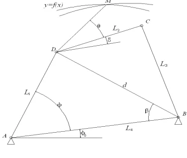
Example 2: Trajectory optimization design of planar four bar mechanism

A given trajectory curve

y

=

f

(x

)

is shown in figure 2 in coordinate system

xoy

.

design a planar four bar mechanism, the connecting point

M

connecting rod curve

y

M

=

f

(

x

M

)

, to fit the best

[image:5.595.209.397.111.270.2]

approximation of curves:

y

=

f

(x

)

.

Fig 2 the trajectories of four-bar mechanism

Tab1 the Coordinate of 10 main points on the path curve

1 2 3 4 5 6 7 8 9 10 xi 9.50 9.00 7.96 5.65 4.36 3.24 3.26 4.79 6.58 9.12

yi 8.26 8.87 9.51 9.94 9.70 9.00 8.36 8.11 8.00 7.89 (1)Determinate design variables

This so-called reproducing the known trajectory, the curve of connecting rod was approximation to a given curve as far as possible. If 10 coordinates of given curve are known in stipulated range, the function of

M

point on the curves of the four bar linkage were shown below:

)

cos(

)

cos(

_{0 5 0}

1

ϕ

+

ϕ

+

θ

+

δ

+

ϕ

+

=

x

l

l

x

_{M A}

)

sin(

)

sin(

_{0 5 0}

1

ϕ

+

ϕ

+

θ

+

δ

+

ϕ

+

=

y

l

l

y

_{M A}

Here:

ϕ

cos

2

₁₄

2 4 2

1

l

l

l

l

d

=

+

−

d

l

ϕ

β

=

arcsin

1

sin

β

δ

=

+

−

−

d

l

l

d

l

2 2 3 2 2 2

2

arccos

Therefore, the coordinate linkage point M is confirm by rod lengths

l

₁,

l

₂,

l

₃,

l

₄,

l

₅, the coordinate of point A

A

x

,

y

_A, and anger

θ

,

ϕ

₀ ; anger

δ

is also expressed by other variables, not as the design variables, so the determine design variables is :

T A

A T

y

x

l

l

l

l

l

x

x

x

x

x

x

x

x

x

X

=

[

1

,

2

,

3

,

4

,

5

,

6

,

7

,

8

,

9

]

=

[

1

,

2

,

3

,

4

,

5

,

,

,

θ

,

ϕ

0

]

(2)establish the target formula

The actual curve of the link point M on the four-bar linkage mechanisms is depicts

y

_M

=

f

(

x

_M

)

, which is the best

approximation of curves

y

=

f

(x

)

, and the formula of target:

2 / 1 10

1

2 2

]

)

(

)

[(

)

(

min

∑

=

−

+

−

=

i

i Mi i

Mi

x

y

y

x

x

f

(3)establish the constraints

Establishing the variable boundary conditions, also the upper and lower

]

57

.

1

,

57

.

1

,

10

,

10

,

,

10

,

10

,

10

,

10

,

5

[

]

,

,

,

[

1 2 9

=

=

u u u

u

x

x

x

]

57

.

1

,

0

,

0

,

0

,

1

,

1

,

1

,

1

,

5

.

0

[

]

,

,

,

[

1 2 9

=

−

=

i i i

i

x

x

x

X

L

So the boundary constraints:

9

,

,

2

,

1

,

0

)

1

2

(

i

−

=

x

−

x

≤

i

=

L

g

_{i ui}

9

,

,

2

,

1

,

0

)

2

(

i

=

x

−

x

≤

i

=

L

g

_{li i}

Considering the existing conditions of the crank, the performance constraint function:

0

)

(

1 2 3 4

1

x

=

x

+

x

−

x

−

x

≤

g

0

)

(

1 3 2 4

2

x

=

x

+

x

−

x

−

x

≤

g

0

)

(

1 4 2 3

3

x

=

x

+

x

−

x

−

x

≤

g

Considering the minimum transmission angle, the constraint functions:

0

2

)

(

arccos

30

)

(

3 2 2 1 4 2 3 2 2 4

≤

−

−

+

−

°

=

x

x

x

x

x

x

x

g

0

150

2

)

(

arccos

)

(

3 2 2 1 4 2 3 2 2

5

−

°

≤

+

−

+

=

x

x

x

x

x

x

x

g

To sum up, the path optimization mathematical model of planar four bar mechanism:

2 / 1 10 1 2 2

]

)

(

)

[(

)

(

min

∑

=

−

+

−

=

i i Mi i

Mi

x

y

y

x

x

f

9

,

,

2

,

1

,

0

)

1

2

(

i

−

=

x

−

x

≤

i

=

_L

g

_{i ui}

9

,

,

2

,

1

,

0

)

2

(

i

=

x

−

x

≤

i

=

_L

g

_{li i}

0

)

(

_{1 2 3 4}

1

x

=

x

+

x

−

x

−

x

≤

g

0

)

(

_{1 3 2 4}

2

x

=

x

+

x

−

x

−

x

≤

g

0

)

(

_{1 4 2 3}

3

x

=

x

+

x

−

x

−

x

≤

g

0

2

)

(

arccos

30

)

(

3 2 2 1 4 2 3 2 2 4

≤

−

−

+

−

°

=

x

x

x

x

x

x

x

g

0

150

2

)

(

arccos

)

(

3 2 2 1 4 2 3 2 2

5

−

°

≤

+

−

+

=

x

x

x

x

x

x

x

g

The trajectory mathematical model of planar four bar mechanism for optimization design is reproduced by Ant algorithm, the solution is found by MATLAB software, and the persistence parameter

α

=

β

=

1

，

r

=

1

，

6

.

0

=

ρ

，

Q

=

1

, iteration number 10, the program runs to get the optimal solution of the ant algorithm

optimization

4127

.

10

)

(

X

=

f

]

7669

.

0

,

8273

.

0

,

9393

.

6

,

6098

.

3

,

7363

.

3

,

0580

.

6

,

5588

.

4

,

2329

.

6

,

5748

.

2

[

−

=

X

The optimum solution was obtained by conventional optimization method [37]:

4133

.

128

)

(

X

=

f

]

22684

.

1

,

37909

.

1

,

24866

.

2

,

06582

.

2

,

97325

.

7

,

03039

.

7

,

40658

.

5

,

81944

.

5

,

67756

.

1

[

=

X

90509

.

11

)

(

X

=

f

]

07579

.

0

,

56984

.

1

,

05477

.

9

,

24869

.

7

,

06242

.

1

,

56997

.

8

,

99993

.

9

,

3485

.

4

,

75864

.

1

[

=

X

So, compared with conventional optimum algorithm and genetic algorithm, the results of the optimization design by Ant algorithm are more advantages, better solution.

Cellular ant algorithm 1)Cellular automata theory

Cellular Automata (CA) is a discrete grid power model in time, space and state. Its basic components include cellular, Cellular space, neighbor, and rules. Simply speaking, Cellular automata can be regarded as a cellular space and the transformation function on this space. Expressed in mathematical symbols, standard cellular automata are four tulles:

)

,

,

,

(

L

S

N

f

A

=

d

A is a cellular automaton system,

L

is a cellular space,

d

is a Cellular automata in cellular space dimensions, is a

positive integer,

S

is a cellular state set, its state is in binary form

{ }

0

,

1

, or discrete set of

integer

{

s

₀

,

_L

,

s

_i

,

_L

,

s

_k

}

,

N

is a combination of the central cell, including the cells in all areas,

f

is a transition function mapped from

S

N to

S

. All cellular cells are located in the

d

dimensional space, the position of them can

be determined by

d

dimensional in integer matrix

Z

d.

Cellular automata are described and defined strict from the perspective of set theory. Symbol

d

is spatial dimensions, symbol

k

is the cellular state, symbol

S

is a finite set,

r

is cellular neighborhood radius,

Z

is a set of integers in one dimensional space, t is the time.

In order to simplified describing and understanding, the cellular automata considers in one-dimensional space

1

=

d

, the whole cellular space is one-dimensional

Z

, and integer set

S

distributed on the state set is written as

S

Z.

1

:

→

t₊ Z

t

S

S

F

The dynamic evolution of the function is determined by various cellular local evolution rules

f

, and usually called

the local rule. Cellular and its neighbors can be written as

S

2r+1 in the one-dimensional space. Local function can be written as:

1 1

2

:

S

_tr+

→

S

_t+

f

Input and output function set are finite sets in the local rules

f

, they are limited reference table. Cellular can obtain

the global evolution applied the local function in cellular space:

)

,

,

,

,

(

)

(

c

_ti₁

f

c

_ti r

c

_ti

c

_ti r

F

₊

=

−

L

L

+

Among: This is a cellular automata model and

c

_tiis a cellular at the position

i

.

2)Cellular ant algorithm and its implementation

Cellular automation is made of a cellular space and transformation function in this space.

Definition 1: continuous function

f

(

x

1

,

x

2

,

L

,

x

n

)

definition domain into a set of

n

Euclidean space, denoted

Definition 2: cellular neighbors described by extended Moore neighborhood

{

}

{

}





_



















∈

≤

−

+

+

−

+

+

−

=

=

× × ×

× ×

×

n n i j i i

ni n i ji

j i i

i

ni ji i

i

Moore

Z

x

x

x

x

x

x

x

x

x

x

x

x

c

N

L

L

L

L

L

L

,

,

,

,

,

,

1 1 1

1

γ

Among them,

x

_i×1

,

L

,

x

_i×j

,

L

,

x

_i×nare the geographical coordinates of neighbor cell values.

Definition 3: cellular ant search

N

_i is an area of cellular space and extended Moore neighbor

r

depends on the

value of the function in definition domain range and number of ants.

Definition 4: area

N

_i refers to the region that is outside the region of the cellular space.

Definition 5: ants transfer probability is defined as follow:

∑

∆

∆

=

k

ik k

ij j

ij

Z

Z

P

_{α β}

β α

τ

τ

)

(

)

(

)

(

)

(

Among them:

τ

_jis attract field strength of ant

j

;

∆

Z

_ijis the objective function values

Z

_i

−

Z

_j;

α

is the relative

importance of trajectory (

α

≥

0

);

β

is the relative importance (

β

≥

0

).

Definition 6: the pheromone updates equation:

=

+

∑

∆

k k i old

i new

i

ρτ

τ

τ

Among them:

∆

τ

_ikis the length of trajectory information left ants

k

in the field

i

units in number, here,

∆

τ

_ikis the

field of mobile value increase

Q

(

Q

is the embodiment of ants leave a constant track number).

ρ

is durable

trajectory (

0

≤

ρ

<

1

).

Definition 7: evolution rule of Cellular:

(1) Selecting any one cell

c

_i, calculating

Z

=

f

(

x

₁

,

x

₂

,

_L

,

x

_n

)

, and recording

Z

_opt

=

Z

,

c

_opt

=

c

_i.

(2) Selecting any cellular

c

_i and

c

_jfrom

N

_i, and calculating

Z

_iand

Z

_j. If the condition is met,

Z

_i

<

Z

_j,

j opt

Z

Z

<

,

∆

τ

k_j increases with the value of

Q

. When

∆

Z

_ij

<

0

, the ant

i

moves to the field

j

with the

probability of

P

_ij, and the region

N

_ideath; when

∆

Z

_ij

≥

0

, the ant

i

continues to search in the area

N

_i.

Since the computational complexity of the algorithm has a relationship with partitioning of cellular space, it uses the method of equilibrium partitioning cellular space to deal with practical problems, which can reduce the computation time. Each region is composed of cellular and cellular neighbor, the center one is cellular in the region, and the rest are neighbors, the cellular and its neighbor state determines the region which is the life or death. Combine with local characteristic functions in the region (local monotone, then the local convexity function), and generate a random number to search local optimal solution by computer. Expand the field outside the cellular space to prevent the algorithm from converging to local optimal solution, transfer area mobility of ants, conducive to global optimization. The implementation steps of cellular ant algorithm:

Step 1

nc

←

0

(

nc

is the number of iterations or search times)

i

τ

_and

∆

τ

i _{initialization}

Determine the area size according to the number and the size of the space of ants, put the ants in the center of the search area;

Step 2 Put the initial of each ant starting point into the current solution concentration

If the moving is successful, then regional

N

i _death;

Step 3 Calculate the objective value

Z

k _{of each ant, and record the best solution}

Step 4 Modify trajectory strength by update equations

Step 5 Each ant

i

:

∆

τ

i

←

0

；

nc

←

nc

+

1

Step 6 if

nc

<

scheduled iterations number and no degradation behavior (i.e., find all the same solution), then go to step 2

Step 7 The best solution to the current output

As can be seen, with the regional life evolution, ants will be concentrated in certain areas, speed up the optimization process.

3)Calculation example

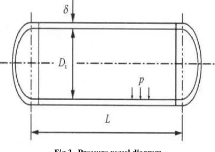
Example: the optimum design of pressure vessel

Cylindrical horizontal pressure vessel design a standard elliptical head, pressure vessel diagram as shown in figure 3. In the premise of the design requirements, to optimize the design of structure parameters, the container weight is the

lightest, supplies at least. Calculation of pressure vessel

P

c

=

1

.

6

MPa

_{, known full volume}

V

=

100m

3_{, material}

in the design temperature of allowable stress

MPa

t

163

]

[

σ

=

_{, limiting yield at the test}

[image:9.595.200.411.409.558.2]

temperature

σ

s

=

345

MPa

_{, the coefficient of welding joint}

φ

=

0

.

85

_{, corrosion allowance}

C

2

=

1

mm

Fig 3 Pressure vessel diagram

(1)Determination of design variables

Quality of pressure vessel shell is determined by the diameter

D

_i, the length of the cylinder

L

and the wall

thickness of the

δ

. For a given volume of pressure vessel design, the length of the tube body can be expressed as a function of the inner diameter of the cylinder body, therefore, selection of tube diameter, tube diameter, tube wall thickness and the head of the wall thickness as the design variables. In design condition, standard elliptical head wall thickness and the wall thickness of the cylinder is connected with roughly equal, in order to make convenient for taking the same value. Therefore, to determine the design variables:

]

,

[

]

,

[

x

₁

x

₂

D

_i

δ

X

=

=

(2) Establishing objective function

Pressure vessel having a cylindrical body and standard elliptical head, the quality

M

of housing is equal to the cylindrical portion (including head straight edge) quality and two head quality

M

₁ and

M

₂.

δ

δ

ρπ

D

L

M

1

=

(

i

+

)

]

)

4

(

)

2

[(

12

3 2

2

D

i

D

i

D

i

M

=

π

ρ

+

δ

+

δ

−

So：

[(

2

)

(

4

)

]

12

1

)

(

2 3

2

1

M

D

i

L

D

i

D

i

D

i

M

M

=

+

=

ρπ

+

δ

δ

+

ρπ

+

δ

+

δ

−

The volume expression: 2 3

12

1

4

1

i

i

L

D

D

V

=

π

+

π

The result：

3

4

2

i

i

D

D

V

L

=

−

π

The target function:

]

)

4

(

)

2

[(

12

1

)

(

)

(

1 2 13

2 2 1 2

2

1

x

Lx

x

x

x

x

x

x

x

f

=

ρπ

+

+

ρπ

+

+

−

3

4

1

2 1

x

x

V

L

=

−

π

(a)Establish the constraints

(b)Strength condition

According to the provisions of GB150-1998[38]，the corresponding thickness formula for cylindrical shell and the

standard ellipsoidal heads must meet.

Cylinder and standard ellipsoidal heads need to satisfy the corresponding thickness formula.

Cylinder: c

t i c

P

D

P

C

C

−

≥

−

−

φ

σ

δ

]

[

2

2 1

Standard elliptical head: c

t i c

P

D

P

C

C

5

.

0

]

[

2

2 1

−

≥

−

−

φ

σ

δ

here：

c

P

——Design pressure

t

]

[

σ

_{——Allowable stress design of material temperature}

1

C

_{——The thickness of the steel plate negative deviation}

2

C

_{——corrosion allowance}

φ

_{——weld joint efficiency}

(c)Minimum thickness

In order to meet the requirements of manufacturing process requirements of stiffness and the transportation and installation process, according to the engineering practice, it provides the minimum thickness requirements which does not include corrosion allowance in GB150-1998[38]

When the cylindrical shell is carbon steel and low alloy

If

D

_i

≤

3800

mm

, then

δ

≥

2

D

_i

/

1000

,

δ

≥

3

mm

(d)Head stability conditions

Effective thickness pressure standard elliptical head by head diameter shall be not less than 0.15%, so:

The effective thickness of standard elliptical head under internal pressure

δ

e

=

δ

−

C

1

−

C

2 _{is not less than 15%}

of the head diameter

D

i _.

0

0015

.

0

2

1

−

−

≥

−

C

C

D

i

δ

(e)Hydrostatic test stress strength condition

Should after pressure test container are made into use, in order to make the hydraulic test container materials are in the elastic state, in the pressure test must be pressed before type checking test cylinder film stress

The container should do pressure test before using, in order to make the hydraulic test container material in the elastic state, it must be check the cylinder film stress formula before the pressure test.

S i T

C

C

C

C

D

P

φσ

δ

δ

9

.

0

)

(

2

)

(

2 1 2 1

≤

−

−

−

−

+

Here： T

P

——test pressure

P

_T

P

_{c t}

]

[

]

[

25

.

1

σ

σ

=

s

σ

——limiting yield under test temperature.

]

[

σ

——the allowable stress of material under test temperature

It induces the mathematical model of optimal design of pressure vessel by the preceding analysis.

]

)

4

(

)

2

[(

12

1

)

(

)

(

min

1 2 13

2 2 1 2

2

1

x

Lx

x

x

x

x

x

x

x

f

=

ρπ

+

+

ρπ

+

+

−

0

]

[

2

)

(

2 1 2

1

−

+

+

≤

−

=

x

C

C

P

D

P

x

g

c t i c

φ

σ

0

5

.

0

]

[

2

)

(

_{2 1 2}

2

−

+

+

≤

−

=

x

C

C

P

D

P

x

g

c t i c

φ

σ

0

1000

/

2

)

(

1 2

3

x

=

x

−

x

≤

g

0

3

)

(

2

4

x

=

−

x

≤

g

0

0015

.

0

)

(

_{1 2 1 2}

5

x

=

x

−

x

+

C

+

C

≤

g

0

9

.

0

)

(

2

)

(

)

(

2 1 2 2 1 2 1

6

−

≤

−

−

−

−

+

=

S T

C

C

x

C

C

x

x

P

x

g

φσ

It solves the mathematical model of optimal design of pressure vessels with cellular ant algorithm, takes the parameters

in the instance into the equation, takes the persistence parameter

α

=

β

=

1

，

r

=

1

，

ρ

=

0

.

6

，

Q

=

1

，cellular

segmentation number is 10, a total of 100 regions, each central region is the cellular the others are cellular neighbor, outside the area of the part is the area of the field. It can calculate the optimization of cellular ant algorithm.

41

.

20641

)

(

X

=

f

]

4

.

13

,

5

.

2136

[

=

X

It obtains the optimal solution by the conventional optimization method [6]

85

.

32191

)

]

20

,

2000

[

=

X

It obtains the optimal solution by the simulated annealing algorithm [6]:

38

.

21355

)

(

X

=

f

]

91

.

15

,

42

.

2429

[

=

X

Thus, compared with the normal algorithm and simulated annealing algorithm, the cellular ant algorithm optimization design results are better, can achieve more optimal solution

RESULTS AND DISCUSSION

1.Intelligent system compilation of mechanical optimization design

1)The system interface design

The interface is an interface for information interaction between user and system.

Usability and friendliness of the application program depends on the interface design, it should consider the purpose of the application program, the use frequency of program, the experience and expectations of user in interface design. In the main interface view (Fig. 4), two modules are designed using the menu editor, the one is the "common problem of mechanical optimization design", the other is the "help". It takes into account some common problems of the mechanical design in the first module, including optimization design of compression cantilever beam, optimization design of planar four bar mechanism trajectory, optimization design of pressure vessel, optimization design of single stage cylindrical gear reducer, optimization design of two level cylindrical gear reducer, optimization design of worm gear reducer, optimization design of produce box plate, optimization design of bolt group connection, etc.

2. Encapsulate calling MATLAB based on VB

(1)Basic principles

The program of the main interface is designed based on VB, the subprograms of MATLAB are called in many ways, the common and convenient way: using function “shell ()” to call MATLAB application, using ActiveX technology and dynamic link library to realize to call the program. In this paper, MATLAB was call by function “shell ()”. Passing parameters is fixed by reading and writing in this method, using advanced programming language of Visual Basic to edit the original parameters of input and output, MATLAB is adopted to write the M recognition function in the VB development environment, and then wage the optimization calculation

The programs of MATLAB are called to invoke the command based on VB:

Dim X

X = Shell ("…\matlab.m")

In the formula, the above command is directly activated and calculated by MATLAB.

(2)Data transfer from VB to MATLAB.

The system is a high intelligent mechanical optimization computing system, and composed of the MATLAB, VB and other parts. The mathematic model for the design should be established firstly, the parameters which defined in the VB program are transformed from VB to MATLAB, the mathematic model is established to optimization calculate.

(3)Data transfer from MATLAB to VB.

The transfer data is mainly complete the calculation from MATLAB, so it is necessary to send the result data to the VB program reflected by interface.

(4)Details of ANSYS operator based on VB (a) The judgment of ANSYS calculation

Add a timer on the interface, and write the following code: Private Sub Timer1_Timer ()

If Dir ("…vort1.mode") <> "" Then MsgBox ("commutate over") Timer1.Enabled = False

Save the results in the date2 file, notify the user that operation is complete in msgbox dialog box, then VB interface output the results.

(b) remove the last VB executable file

Because of each optimization calculation, the system will produce lots of files in the VB directory, so a kill program (App.Path &"... ") should be added to prevent the originally text files, such as data1, data2, affecting the next operation.

Fig 4. The main interface of mechanical optimization design

3. Application example

Firstly, enter the main interface of system, as shown in figure 4. Select the "optimization design of pressure vessel" in the drop-down list into the pressure vessel design interface, click to enter the data input interface to input the basic parameters of pressure vessel:

Mpa

P

c

=

1

.

6

_,

V

=

100m

3 _,

[

σ

]

t

=

163

Mpa

_,

σ

s

=

345

Mpa

_,

φ

=

0

.

85

_,

C

1

=

0

.

25

_,

C

2

=

1

。

3

/

7850

kg

m

=

ρ

_,

P

T

=

1

.

6

Mpa

_,

[

σ

]

=

163

Mpa

_.

Then, press the save button to generate a text file data1 of pressure vessel parameters in the VB root directory. Press the OK button, select the different optimization algorithm on the pressure vessel design interface, then can get the different optimization results immediately. The calculation results of three kinds of optimization algorithm are shown in table2.

Tab2 Calculation results of 3 kinds of optimization algorithm

Algorithm x1 x2 f(x)

Ant algorithm 2422.2 15.1 20761.11 Cellular ant algorithm 2136.5 13.4 20641.41 Quantum ant colony algorithm 2048.7 12.9 20659.22

CONCLUSION

Several different algorithms are compared, such us: ant algorithm, cellular ant algorithm, and quantum ant colony algorithm. The corresponding mathematical models are established according to the actual mechanical design problems by computer, and the best solution is chosen.

(2) The application of the ant algorithm in optimum design is introduced. While Quantum algorithm and cellular automata are introduced into the ant algorithm, two new optimization algorithms are developed, one is Cellular ant algorithm, the other is Quantum ant colony algorithm. Through the actual project design, these methods are proved to be more useful. Studies in the thesis provide a new approach for mechanical optimization design.

(3) A relatively rich and friendly operation interface is established by Visual Basic, users only need to select the mechanical problems to be solved and enter the known key parameters, then the best result will be output, it greatly facilitate the users, especially for whom don’t understand the intelligent algorithm.

Acknowledgment

This work was financially supported by the Key Laboratory for Advanced Technology in Environmental Protection of Jiangsu Province (AE201039) (AE201038). Natural science foundation of Jiangsu Province（BK2012250. The

Natural Science Foundation for General Universities of Jiangsu Province (China) under Grant No. 12KJD520010.

REFERENCES

[1]Duda J W, Jakiela M J. Genetation and classification of structural topologies with genetic algorithm

speciation[J], 1997, 119(3):127～131.

[2] Franklin Y. Cheng, Dan Li. Genetic algorithm development for multi-objective optimization of structures[J] ,

1998, 36(6):1105～1112.

[3] Nagendra S, Jestin D, Gurdal Z, et al. Improved genetic algorithm for the design of stiffened composite

panels[J]. Computer & Structures, 1996, 58(3):543～555.

[4] Li Quan shui, Gong Yibin, Yang Daoguo, Liang Junsheng. Mechanical structure optimization design based on

Ant Algorithm[J] , 2003, 22(suppl.):131～132,187.

[5] Guo Huixi, Gui Naixin, HeZemin. Ant colony algorithm and its application in mechanical optimal design[J] ,

2005,17(3)：50～52.

[6] Li Zhi, Chen Minyi. Ant colony algorithm and its application in the optimal design in the special spiral groove