Journal of Chemical and Pharmaceutical Research, 2014, 6(9):463-468
Research Article
CODEN(USA) : JCPRC5
ISSN : 0975-7384
Performance comparison of several kinds of improved genetic algorithm
Wang Xue-mei
1, Liu Xiao
2and Liu Gang
11
College of Information Science and Engineering, Henan University of Technology, Zhengzhou, Henan, P. R. China
2Zhengzhou Centre for Communication Technology Co., LTD, Zhengzhou, Henan, P.R. China
_____________________________________________________________________________________________
ABSTRACT
Four kinds of improved genetic algorithm are designed in this paper combining the standard genetic algorithm with the hierarchical strategy and the idea of simulated annealing. They are namely hierarchic genetic algorithm, simulated annealing genetic algorithm and simulated annealing hierarchic genetic algorithm. The availability and the validity of these algorithms have been verified by the calculation results. The further performance analysis of the algorithms proves that not only the global convergence but also the genetic evolution speed are improved through the modified algorithm introduced in this paper.
Key words: Hierarchic Genetic Algorithm, Simulated Annealing Algorithm, Simulated Annealing Hierarchic Genetic Algorithm, Adaptable Genetic Algorithm, Optimization Model
_____________________________________________________________________________________________
INTRODUCTION
Genetic algorithm (GA)is a stochastic optimization method which simulates the evolution of biological
populations. It is of strong robustness and optimization ability, but the standard genetic algorithm does not guarantee the global optimal convergence.[1-2].Generally, the first is premature convergence and the second is the low searching efficiency at later evolution process.
In order to overcome the defects of the standard genetic algorithm, two improved methods have been introduced in this paper. On one hand, it attempts to combine the standard genetic algorithm with other optimization methods organically to fuse the respective advantages of different algorithms; on the other hand, the design of genetic manipulation (for example: coding) of standard genetic algorithm itself is modified to improve its global search capability and convergence performance.
APPLICATION EXAMPLES
The optimization of (N+M) fault-tolerant systems aims at the lowest total cost within the life cycle. The total cost C is the sum of C1 and C2 .Here, C1 is the purchase cost of the controllers, which is related to their amount, reliability and maintainability. C2 is the direct economic loss due to the unreliability of the controllers during the life cycle, and it is related to the nature of the controlling process and the amount of abnormal controllers. Meanwhile, (N+M) fault-tolerant systems satisfy the constraint of guarantee availability[3].
The cost optimization model of (N+M) fault-tolerant systems is as shown in formula (1).
(
)
0 0 0
1 1
( / )
mi n
( / )
j N
M i j
i
K
C λ µ N M K i P
λ µ +
=
= + +
∑
(1)Here,
(
)
(
)
N Mi M i
M M N i
M
C
P +
+ +
+
+ = + λ µ
µ λ
1 ,
(
)
(
)
N MM
i
i i
M N
C
A
= ++
+
=
∑
µ
λ
µ
λ
1
0.
In the preceding equations, N is used to express the amount of working controllers, M is the amount of standby ones, λ/µ indicates the ratio of the failure rate to the repair rate, K0 expresses the price of a single controller when
λ/µ=λ0/µ0 , K1 is the cost we have to pay for the abnormal work in a single process, PM+I indicates the probability when the system is in the (M+i)th state, and A is the availability of the system, G is the guarantee availability.
The above model has the following features:
(1) It is a hybrid optimization problem which includes integer variables and real variables. (2) The objective function and the constraints show high nonlinearity.
(3) The polynomial expressions of the constraints are not fixed. (4) Contour area of the objective function is very narrow. (5) The objective function is multi-peak.
(6)The figure away from the optimal solution is steep.
(7) The figure becomes flat in the vicinity of the optimal solution for each peak. Therefore, to optimization model, it is very difficult to obtain global optimal solution by standard genetic algorithm[4-10].
IMPROVED GENETIC ALGORITHM 3.1 Hierarchic Genetic Algorithm.
The basic idea to solve the problem of premature convergence is to keep the diversity of the individuals in the group. Hierarchical genetic algorithm is divided into N sub populations in a low level, this N genetic algorithms had better have bigger differences on the feature setting, which can generate more types of excellent schema for high-level genetic algorithm while maintaining the excellent individual evolution stability , under the condition of that the population size does not expand.
This algorithm first generate N * n samples randomly (N≥2, n≥2 ), and then divide them into N sub populations. Each population consists of n samples obviously. They run their own genetic algorithm respectively and independently, recording them as GAi ( i= 1, 2,…,N ). After the genetic algorithm of each sub population run to a certain generate, record the results of N genetic algorithms to two-dimensional array R[1 ~ N, 1 ~ n], where R[ i , j] ( i = 1 ~ N, j = 1 ~ n ) indicate the jth individual of the populations in the results of GAi. At the same time, the average fitness values of the N results is recorded in the array A[1 ~ N], where A[i] express the average fitness values of populations in the results of GAi.
High-level genetic algorithm is similar to the standard genetic algorithm in operation. The results will be passed back to the lower genetic algorithm after the algorithm runs to a certain generation. When N GAi run to a certain generation respectively once more, update the array R[1 ~ N, 1 ~ N] and A[1 ~ N] again, and start a second round of high-level genetic algorithm. Followed by reciprocating, until that the satisfied solutions are obtained[11-15].
The low-level genetic algorithm is divided into three sub populations in this paper, and each of them adopts different coding method respectively.
(1)The first sub population and the high-level populations are coded by floating-point method.
(2) The second sub population encodes M (integer variable) using binary coding method, and encodes λ/µ (floating point variable) using floating-point method.
(3) The third sub population is also coded by the binary method. At the same time there are great differences in genetic operation setting of each sub population such as selection, crossover and mutation and so on.
3.2 Simulated Annealing Genetic Algorithm
A. Simulated annealing with constraints
There are usually two methods to deal with the constraints: abandoning the infeasible solution and using the penalty function. The efficiency of the former method is quite low. To the latter method, if the penalty term is excessive, it probably leads to premature convergence.
On the contrary, the convergence is poor. Therefore, a new method of annealing penalty function is introduced in this paper which based on the idea of the simulated annealing algorithm. It adopts the penalty factor of the simulated annealing and its mathematical model is shown in formula (2).
(
)
(
)
< −
+ +
+
≥ +
+ =
∑
∑
= + = +
G A G A T iP K M N K
G A iP
K M N K
C N
i i M j
j
N i
i M j
j
2 1
1 1 0
0 0
1 1 0
0 0
) ( 1 )
/ (
) / (
) / (
) / (
min
µ λ
µ
λ λ µ
µ λ
(2)
Where, T1 is similar to the temperature T in simulated annealing. At the beginning of the evolution process, T1 is relatively high, and the penalty term 1/T1 is correspondingly small, which means that the penalty to the infeasible solutions is less, so some useful infeasible solution can be included in the process of evolution, which benefits the evolution. With the decrease of T1, the penalty term 1/T1 gradually increased along with the process of evolution, and the penalty of the infeasible solutions becomes bigger and bigger, at the same time, the solutions tend to the feasible ones and reach eventually for the optimal solutions.
B. Simulated annealing with crossover probability and mutation probability
The selection of Pc (crossover probability) and Pm (the mutation probability) has direct influence on the convergence of algorithms. At the beginning of the evolution, in order to avoid the premature phenomenon caused by the rapidly propagating of several individuals with high fitness, Pc and Pm Should not be too small to enhance population diversity; On the contrary, in the latter evolution, when individuals are close to the optimal solutions, Pc and Pm should not be too large to avoid that individuals could not reach for the optimal solutions for a long time[17].
Adaptive Pc &Pm are designed in this paper based on the idea of simulated annealing, its functional formulas is as shown in formula (3).
3 . 0 ) 2 1
sin( 2 . 0 )
(
2 2
)
( = − × +
π
gen T
T
p c m (3)
Here, T2 is the reciprocal of the evolutionary generations which is similar to the temperature T in simulated annealing, and gen is the total preset evolutionary generations. At the beginning of the evolution, T2 is high, so Pc and Pm are rather big, which is beneficial to the diversity of the population; T2 decreases gradually with the increase of the evolutionary generations, and Pc & Pm decrease accordingly, so it is convenient for individuals to come close to the optimal solutions.
C. Simulated annealing with crossover and mutation individual
Here, Boltzmann survival mechanism of simulated annealing algorithm is used to solve the problem of genetic algorithm local solutions. It shows that individuals of each generation which is after crossover and mutation need to experience the process of “generating new solutions-judgment-accept/discard” during the course of evolution. The
evolution process can accept the deteriorative solutions with a probability of exp(-
∆
C/bT3) in addition to accept the optimal ones, which is the essence of that the simulated annealing genetic algorithm is better than the standard genetic algorithm to obtain the global solutions. At the beginning of the evolution process, T3 is relatively high, and poor deteriorative solutions are probable; With T3 decreasing gradually, the evolution process can only accept the better deteriorative solutions; At last,T3 approaches to zero, the deteriorative solutions will be not probable. Therefore, the evolution process will stride over the trap of local optimal solutions[18-20].3.3 Design of the simulated annealing hierarchic genetic algorithm
In this paper, a new global search algorithm is designed by combining the simulated annealing genetic algorithm with the hierarchic genetic algorithm, both of which have their respective advantages on overcoming the defects of the standard genetic algorithm.
The hierarchic design method of simulated annealing hierarchic genetic algorithm is almost the same as the design of hierarchic genetic algorithm mentioned above in the 3.1 section. Where they are different is the choice of Pc and Pm, this algorithm adopt the adaptive ones with simulated annealing in the 3.2 section instead of the original fixed ones mentioned in the 3.1 section. Through this, the global performance and the search capability of the algorithm are all improved. In order to exert the merits of hierarchic genetic algorithm, Pc and Pm among three sub populations are different respectively. According to the idea of simulated annealing, adaptive Pc and Pm are designed accordingly.
For the high-level population1 is as shown in formula (4).
( ) 2
2
1
( ) 0 . 2 s i n ( ) 0 . 3
2
c m
p T
T g e n e r a t i o n π
= − +
× (4)
For the sub population 2 is as shown in formula (5).
( ) 2
2 1
( )= −0.3 +0.4
×
c m
p T
T generation
(5)
For the sub population 3, Pc and Pm are fixed value of 0.3.
THE RESULTS OF SOLUTION AND PERFORMANCE ANALYSIS 4.1 The results of solution
In the above system, respectively choosing N=1,2,…,24, the solutions of M and λ/µ calculated by the
[image:5.595.170.441.387.477.2]programs of simulated annealing genetic algorithm show in the below TABLE I:
Table I. Solutions of optimization
N M λ/µ N M λ/µ N M λ/µ N M λ/µ
1 1 0.00374 7 2 0.007864 13 4 0.024685 19 5 0.029256 2 1 0.002683 8 3 0.018540 14 4 0.023415 20 5 0.028153 3 1 0.002211 9 5 0.029256 15 4 0.022287 21 5 0.027141 4 2 0.010976 10 5 0.028153 16 4 0.021278 22 6 0.036984 5 2 0.009624 11 5 0.027141 17 5 0.031778 23 6 0.035744 6 2 0.008632 12 6 0.036984 18 5 0.030458 24 6 0.034591
4.2 Performance analysis of several genetic algorithms
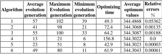
In order to compare the performance of different algorithm, six kinds of algorithms are designed in this paper. Performance indicators of six different algorithm show in the below TABLE II.
Algorithm 1: standard genetic algorithm, Pc = 0.3, Pm = 0.3, the constraints are processed by abandoning the infeasible solutions; Algorithm 2: hierarchical genetic algorithm, Pc = 0.3, Pm = 0.3, the method of constraint processing is the same as algorithm 1; Algorithm 3: hierarchical genetic algorithm, Pc = 0.3, Pm = 0.3, but we adopt the method of annealing penalty function to process the constraints; Algorithm 4: simulated annealing genetic algorithm, the choosing of Pc and Pm is the same as the method mentioned in section 3.2, and the method to process the constraints is also by abandoning the infeasible solutions; Algorithm 5: simulated annealing genetic algorithm, Pc and Pm are same as the ones mentioned in section 3.2, the method of constraints processing is same to algorithm 3; Algorithm 6: simulated annealing hierarchical genetic algorithm, Pc and Pm are the ones mentioned in section 3.3, we also adopt the method of annealing penalty function to process the constraints.
Table II. Performance indicators of different algorithm
Algorithm
Average evolution generation
Maximum Evolution generation
Minimum evolution generation
Optimizing time
Average optimum
values
Relative errors
%
1 57 102 39 49.3 344.4868 0.05362
2 41 98 21 72.4 344.3068 0.00135
3 55 100 33 64.2 344.3087 0.00188
4 13 21 6 156.8 344.3022 0.0
5 23 51 8 42.9 344.3023 0.00003
6 49 80 11 61.9 344.3043 0.00061
The performance parameters showed in table 2 are gained when N is equal to 20. In this condition, the optimum value of M is 5 through looking up the table 1.The actual optimal value λ/µ can be obtained through the iterative method under the condition that N and M are sure. The actual optimum fitness value can also be obtained at the same time and is 344.3022.
(1) The optimum fitness values obtained from the later five kinds of algorithms are all superior to the standard genetic algorithm, which shows that the modified genetic algorithms have improved in search capability.
(2) The convergence time of algorithm 2 and algorithm 4 are respectively longer than algorithm 3 and algorithm 5, and this indicates that the convergence efficiency of the method of abandoning infeasible solutions is inferior to the method of annealing penalty function; But the convergence accuracy of the former two algorithms are respectively higher to the latter ones, which means that the search capability of the first method is better than the second one.
(3) From that the errors obtained from algorithm 4 and algorithm 5 are obviously less than the values gained from algorithm 2 and algorithm 3 , we can see the performance of the algorithm combined with simulated annealing algorithm is better than that combined with hierarchical strategy.
CONCLUSION
The innovation points of this paper embody as follows: (1) Three kinds of improved genetic algorithms are designed combining the standard genetic algorithm with the hierarchical strategy and the idea of simulated annealing. (2) Genetic operations are also designed to make the three sub populations have genetic strategies with great difference. (3) The standard genetic algorithm is immerged into annealing strategy from three aspects, which is beneficial to improve its global optimizing ability. Algorithm analysis shows that both the hierarchical strategy and the simulated annealing strategy are all improvement to the standard genetic algorithm in efficiency.
REFERENCES
[1]Debao Chen, Chunxia Zhao. Acta Scientiarum Naturallum (Universitatis Nakaiensis), vol. 38-6, pp.84-88, 2005. [2]Lijia Xu, Haibo Pu, Hongjian Jiang. Journal of Microcomputer information,vol. 2-2, pp.251-253, 2006.
[3] Luqing Ye,Shengtie Wang. IEEE Transactions on Power Systems,vol. 16-3, pp.340-345, 2001.
[4]Chaogai Xue, Lili Dong, Guohua Li. Journal of Software, Vol 6, No 3, pp. 436-443, Mar 2011. [5]Dongsheng Liu, Journal of Software, Vol 5, No 11, pp. 1243-1249, Nov 2010.
[6]Yongheng Chen, Wanli Zuo, Fengling He, Kerui Chen Journal of Software, Vol 6, No 9, pp. 1655-1663, Sep 2011.
[7]Shaomei Yang, Qian Zhu, Zhibin Liu Journal of Software, Vol 7, No 3, pp. 620-625, Mar 2012.
[8]Yannis E. Ioannidis and Eugene Wong, In Proceedings of the 1987 ACM SIGMOD international conference on Management of data, vol. 16, pp.9-22, 1987.
[9]Jun Deng, Gang Li, Yibing Li, A Study of Application of Simulated Annealing Algorithms to Over all Planning of Land Uses [J], the science and technology management of country’s territory resources, pp: 101-103, June 2007. [10]Daojie Liu, The Simulated Annealing Algorithm Used in Forecasting the Production Capacity of a Steam-Stimulated Well [J], Computer Applications of Petroleum Vol. 15, No. 4, pp: 32-37,2007.
[11]Yian Liu, Jing Liu, Jie Wu, Xiaohua Zou, Application of Simulated Annealing Algorithm in Turning Angle to Avoid Collision Between Ships [J], Shipbuilding of China, Vo l. 48, No. 4 , pp: 53-57, Dec. 2007.
[12]Jianqin Ma, Hui Zhou, Lin Qiu, Bo Zhou, Neural Network Based on Simulated Annealing Algorithm and Back Propagation and Application in the Groundwater Level Forecast of Irrigation District [J], Journal of North China Institute of Water Conservancy and Hydroelectric Power, Vol. 28 No. 6, pp:4-6, Dec. 2007.
[13]Wolfgang Scheufele and Guido Moerkotte, In ACM SIGACT-SIGMOD-SIGART Symposium on Principles of Database Systems, pp.238-248, 1997.
[14]Dagli C H,Hajakbari. In Proceedings of IEEE International Conference on Systems, Man and Cybernetics, 1990, pp.221-223.
[15]Liu Haidi, Yang Yi, Ma Shengfeng, and Li Lian, Journal of Computer Research and Development,vol. 45-1, pp.35-39, 2008.
[16]Zhang Juanqing , Sun Wei, Journal of Southeast University (Natural Science Edition),vol. 34, pp.207-210, 2004.
[17]LIU Jichun, ZHANG Peng, WU Lei, YANG Liu, Journal of Power System Technology,vol.35-8,pp.30-34, 2011. [18]WEI Lian - w e i, SHAO Jing - li, ZHANG Jian-li, CUI Ya-li, Journal of Ji lin University( Earth Science Edition ),vol. 34-4, pp.612-616, 2004.