Finding the Asymptotically Optimal Baire Distance for Multi Channel Data

(1)

http://dx.doi.org/10.4236/am.2015.63046

Finding the Asymptotically Optimal Baire

Distance for Multi-Channel Data

Patrick Erik Bradley

1

_{, Andreas Christian Braun}

2

1_{Institute of Photogrammetry and Remote Sensing, Karlsruhe Institute of Technology, Karlsruhe, Germany} 2_{Remote Sensing and Landscape Information Systems, University of Freiburg, Freiburg, Germany}

Email: [email protected], [email protected]

Received 16 February 2015; accepted 6 March 2015; published 10 March 2015

This work is licensed under the Creative Commons Attribution International License (CC BY). http://creativecommons.org/licenses/by/4.0/

Abstract

A novel permutation-dependent Baire distance is introduced for multi-channel data. The optimal permutation is given by minimizing the sum of these pairwise distances. It is shown that for most practical cases the minimum is attained by a new gradient descent algorithm introduced in this article. It is of biquadratic time complexity: Both quadratic in number of channels and in size of data. The optimal permutation allows us to introduce a novel Baire-distance kernel Support Vec-tor Machine (SVM). Applied to benchmark hyperspectral remote sensing data, this new SVM pro-duces results which are comparable with the classical linear SVM, but with higher kernel target alignment.

Keywords

p-Adic Numbers, Ultrametrics, Baire Distance, Support Vector Machine, Classification

1. Introduction

The Baire distance was introduced to classification in order to produce clusters by grouping data in “bins” by [1]. In this way, they seek to find inherent hierarchical structure in data defined by their features. Now, if there are many different features associated with data, then it is reasonable to sort the feature vector by some criterion which ranks their contribution to this inherent hierarchical structure. We will see that there is a natural Baire distance associated to any given permutation of features. Hence, it is natural to ask for this task to be performed in reasonable time. In general, there is no efficient way of sorting n variables, but if the task is to find a permutation satisfying some optimality condition, then often a gradient descent algorithm can be applied. In that case, the run-time complexity is decreased considerably.

(2)

linear cost function depending on the pairwise Baire distances for all possible permutations. The Baire distance we use depends on a parapmeter , and we argue that the precise value of this parameter is seldom to be expected of interest. On the contrary, we believe that it practically makes more sense to vary this parameter and to study the limiting case →0. Our theoretical result is that there is a gradient-descent algorithm which can find the asymptotic minimum for →0 with a runtime complexity of _{O dn}

( )

2 _{, where}

d is the number of

all data pairs.

The Support Vector Machine (SVM) is a well known technique for kernel based classification. In kernel based classification, the similarity between input data is modelled by kernel functions. These functions are em- ployed to produce kernel matrices. Kernel matrices can be seen as similarity matrices of the input data in reproducing kernel Hilbert spaces. Via optimization of a Lagrangian minimization problem, a subset of input points is found, which is used to produce a separating hyperplane for the data of various classes. The final de- cision function is dependent only on the position of these data in the feature space and does not require esti- mation of first or second order statistics on the data. The user has a lot of freedom on how to produce the kernel functions. This offers the option of producing individual kernel functions for the data.

As an application of our theoretical result, we introduce the new class of Baire-distance kernels which are functions of our parametrized Baire distance. For the asymptotically optimal permutation, the resulting Baire distance SVM yields results comparable with the classical linear SVM on the AVIS Indian Pine dataset. The latter is a well known hyperspectral remote sensing dataset. Furthermore, the kernel target alignment [2] represents an a priori quality assessment and favours our new Baire distance multi-kernel SVM constructed from Baire distance kernels at difference feature resolutions. This new multi-kernel combines in a sense our first approach with the approach of [1], as it combines the different resolutions defined by their method of “bin” grouping. As our preliminary practical result, we obtain greater completeness in many of our clusters than with the classical linear SVM clusters.

2. Ultrametric Distances for Multi-Channel Data

After a short review on the ultrametric parametrized Baire distance, it is shown how to find for n variables their asymptotically optimal permutation for a linear cost function defined by permutation-dependent Baire distances. It has quadratic run-time complexity, if the data size is fixed.

2.1. Baire Distance

Let x y, be words over an Alphabet A. Then theBaire distance is

( )

( ),

, 2 x y d x y = −

where 

(

x y,

)

is the length of the longest common initial subword, as depicted in Figure 1. The length of a word is defined as the number of letters from A (with multiple occurrences). The reason for choosing 1

2 as

the basis in the Baire distance is pure arbitrariness, at least to our opinion. Hence, 1

2 can be replaced by any fixed  in the interval

( )

0,1 .

Definition 2.1. The expression

(3)

( )

( ),

, x y

d_ x y = is the -Baire distance.

Later on, we will study the limiting case →0.

Remark 2.2. The metrics d are all equivalent in the sense that they generate the same topologies.

The Baire distance is important for classification, because it is an ultrametric. In particular, the strict triangle inequality

( )

, max

{

( ) ( )

, , ,

}

d x y ≤ d x z d z y

holds true. This is shown to lead to efficient hierarchical classification with good classification results [1] [3] [4].

Data representation is often related to some choice of alphabet. For instance, the distinction “Low” and “High” leads to A=

{ }

0,1 and is used in [4]. The decimal representation of numbers yields A=

{

0,1,, 9

}

for the method in [1]. A very general encoding with arithmetic flavour is given by subsets A⊆O_K inside the ring of integers inside a p-adic number field K, with all a∈A different modulo [5]. No knowledge of p-adic number theory is required for what comes after the following Example 2.3. However, the interested reader may consult [6] for a first application of such mathematics in classification.

Example 2.3. The simplest example of p-adic number fields K in data representation is given by taking K as the field of 2-adic numbers . Then O_K =₂ is the ring of 2-adic integers, and as alphabet A=

{ }

0,1 . The numbers 0.1 represent the finite field ₂ in a standard way which is often used when 2-adic numbers are written out as power series in 2, i.e. as finite or infinite binary numbers.

The role of the parameter  in classification can be described as follows. Let X ⊆A be a set of words.

Then X defines a unique dendrogram D X

( )

, and d_ defines a metric dendrogram D_

( )

X =

(

D X

( )

,d_

)

. Observe that D_

( )

X depends only on the metric d_. By equivalence of the Baire metrics, dendrograms D_

( )

X are tree-isomorphic for all . However, optimal classification results in general do depend on , as has been observed in Theorem 2 of [7], where the result is formulated for p-adic ultrametrics.

2.2. Optimal Baire Distance

Given data X and attributes p=

(

p₁,,p_n

)

with possible values V =

{

v₁,,v_m

}

, then a permutation σ ∈S_n, where S_n is the symmetric group of all permutations of the set

{

1,,n

}

, defines the expression

( )

: ( )1

( )

( )2

( )

( )n

( )

pσ x = p_σ x p_σ x p_σ x

i.e. a word with letters from the alphabet V . This yields the Baire distance d_σ

( )

x y, .

In order to determine a suitable permutation for the data, consider the average Baire distance. A high average Baire distance will arise if there is a large number of singletons, and branching is high up in the hierarchy. On the other hand, if there are lots of common initial features, then the average Baire distance will be low. In that case, clusters tend to have a high density, and there are few singletons. From these considerations, it follows that the task is to find a permutation σ ∈S_n such that

( )

(

)

,

, x y X

Eσ dσ x y

∈

=

∑

_



is minimal, leading to the optimal Baire distance d_σ. Any method attempting to fulfil this task must overcome the problem that S_n =n! is quite large for large n.

Let P=

(

p₁,,p_n

)

, written as

{

1,,n

}

. Expanding Eσ

( )

 into powers of  yields:

( )

_{( )}

0 0

,

k

n n

J k J

E with m

ν

σ σ ν σ

ν ν σ

ν=α α = ∈Σ

=

∑

=

∑ ∑

  (1)

(4)

( )

{

2 ,

}

k P

J J k J

ν λ ν

Σ = ∈ = = (2)

where J=

{

j₁<< j_k

}

, and

( )

(

)

1 k, 1

j j n

J w w w w

λ =   is the length of the common initial subword with

the standard word w₁w_n obtained by defining an ordering on any arbitrary alphabet A=

{

w₁,,w_n

}

. Some first properties of k

ν

Σ are listed in the following: 1. k

ν

Σ = ∅ if

ν

>k 2. Σ = ∅00

{ }

3. 1

{

{ } { }

{ }

}

0 2 , 3 , , n

Σ = 

4. 2

{

{ }

{ } { }

{ }

{

}

0 2, 3 , , 2,n ; 3, 4 , , 3,n ; , n 1,n

Σ =    −

5. Σ =n_n

{

1,,n

}

These properties follow from Equation (2) above, and they imply some first properties of α_νσ:

{ }

( ) ({ }) ({ })

0 , , ,

1 i 2 i j 2 i j k

i i j n i j k n

m m m m

σ

σ σ σ

α _∅

≠ ≤ < ≤ ≤ < < ≤

= +

∑

+

∑

+

∑

+ (3)

( ) ( )

{ }

1 1 , , 1

n m n

σ

σ σ

α ₋ = _ ₋ (4)

{1, ,}

n m n

σ

α = _ (5)

An important observation is that α_νσ depends only on the first ν+1 permuted values σ

( )

1 ,,σ ν

(

+1

)

. This will be exploited in the following section, where it is shown how optimal permutations σ can be computed.

The following two examples list all values of

( ) , : k k J J m ν σ ν σ α ∈Σ =

∑

in the case

σ

=id for n=3, 4. By effecting the permutation σ , one obtains the corresponding matrices

( )

,k σ ν

α , and summing over the row labelled ν yields α_νσ. Example 2.4. Table for n=3 and

σ

=id:

{ } { } { }

{ } { }

{ }

2 3 2,3

1 1,3

1,2

1,2,3

3 0 1 2 3

0

1

2

3 n

m m m m

m m m m ∅ = +

Example 2.5. Table for n=4 and

σ

=id:

{ } { } { } { } { } { } { }

{ } { } { } { }

{ } { }

{ }

2 3 4 2,3 2,4 3,4 2,3,4

1 1,3 1,4 1,3,4

1,2 1,2,4

1,2,3

1,2,3,4

4 0 1 2 3 4

0 1 2 3 4 n

m m m m m m m m

m m m m

m m m m ∅ = + + + + +

2.3. Finding Optimal Permutations

(5)

The function

( )

0

Eσ _νσ ν

ν

α

≥

=

∑

 

from Equation (1) is to be minimised, where σ ∈S_n is a permutation of the set N. A combinatorialtopo- logical point of view appears to be helpful in the task. Namely, view the simplex ∆ as a (combinatorial) simplicial complex. A star of an i-face x∈ ∆ is the set of ν -faces attached to x with ν ≥i (including x itself). The weak topology on ∆ is generated by the stars.

To ∆ is associated a graph Γ_∆ whose vertices are the faces, and an edge is given by a pair

(

v v, ′

)

consisting of an i-face v and an i+1-face v′ such that v is a face of v′.

The counts m_J_{( )}_σ appearing in Equation (1) define a function m:P

( )

N →N, and this in turn yields weights on Γ_∆ in the following way:

( )

(

)

Star vertex weights U U v

w v m

∈

=

∑

(6)

( )

, if

(

,

)(

edge weights

)

w e =w v −w v′ e= v v′ (7)

Observe that all edge weights are non-negative:

( )

0 w e ≥

because Star

( )

v′ ⊆Star

( )

v . The graph Γ_∆ is a directed acyclic graph with origin vertex v∅ and terminal vertex v_N.

An injective path γ:v∅vJ in Γ∆ has a natural -length

( )

1

( )

0 w e ν µ µ µ γ − = =

∑

 

where γ is given by the sequence of edges

(

e₀,,e_ν−₁

)

.

Definition 2.6. A permutation σ ∈S_n is said to be compatible with an injective path γ:v∅ vJ, if

( )

{

σ i

}

=Ji\Ji−1 (8)

where γ is given by the sequence of sets J₀ = ∅,,J_ν =J. Lemma 2.7. If σ is compatible with γ, then

( )

1

0 ν

σ µ µ µ

γ −α

=

∑

 

where the path γ is given as in Definition 2.6.

Proof. Let e_µ =

(

v v_µ, _µ₊₁

)

be an edge on γ given by the pair of sets J_µ, J_µ₊₁. Then

( )

( ) ( )1

Star \Star

u

U v v

w e m

µ µ

µ

+

∈

=

∑

Assume that

σ

=id is compatible with γ . Then

( )

1

{

}

0

Star \ Star 2 1, , , 1

n

N k

k

v_µ v_µ+ I I µ µ I _µ

=

= ⊆ ⊇  + ∈/ =



Σ (9)

from which the assertion follows for

σ

=id by summation over the edges along γ. For arbitrary σ compatible with γ the proof is analogue to this case.

The following is an immediate consequence:

Corollary 2.8. Let γ :v∅vN, and σ compatible with γ . Then

( )

N

( )

N

m Eσ

γ

+ =

  

(6)

Corollary 2.9. Dijkstra’s shortest path algorithm on Γ_∆ finds the global minima for Eσ

( )

 with any given

( )

0,1

∈

 .

The main problem with applying Corollary 2.9 is the size of Γ_∆ for large n. However, we believe that it is of practical interest to consider Eσ

( )

 for sufficiently small . We will show below that in this case, the following gradient descent finds the global minimum in an exhaustive manner. Given an edge e=

(

v w,

)

, the expression o e

( )

will denote the origin vertex v, and t e

( )

means the terminal vertex w.

Algorithm 2.10. (Gradient descent) Input.

(

Γ_∆,w

)

. Step 0. Set V₀:=

{ }

v_∅ and E₀ =

{

all edges of Γ_∆

}

.

Step 1. Collect in E₁ all edges e with o e

( )

∈V₀ having smallest weight w e

( )

, and set V₁:=

{

t e e

( )

∈E₁

}

.

Step ν>1. Collect in E_ν all edges e∈E_{ν −}₁ with o e

( )

∈V_ν−₁ having smallest weight, and set

( )

{

}

:

V_ν = t e e∈E_ν .

Output. The subgraph of Γ_∆ containing all paths with smallest sum of edge weights from v∅ to vN. This algorithm clearly terminates after n steps. The paths γ:v∅ vN correspond bijectively to a set  of permutations σ ∈S_n.

Lemma 2.11. Let σ∈ be a permutation derived from gradient descent, ∈

( )

0,1 , and τ ∈S_n such that

( )

Eτ  is minimal. Then there exists a constant C_τ >0 such that for all 0< <η C_τ it holds true that

( )

Eσ

η

≤Eτ

η

.

Proof. We may assume that there exists some ν∈

{

1,,n

}

such that

τ σ

ν ν

α <α (10)

as otherwise Cτ := can be chosen. Assume now further that ν be minimal with property (10). Still further, we may assume that there exists some µ∈

{

1,,ν−1

}

such that

σ τ

µ µ

α

<

α

(11)

as otherwise σ could not be derived by gradient descent. The reason is that at step ν that method would descend down to τ ν

( )

instead of to σ ν

( )

, since ν is the first occurrence of property (10). Let now µ be minimal with (11). All this implies that

( )

E

( )

t E

( )

t P t

t

τ σ

τ µ

− =

is a polynomial with real coefficients such that P_τ

( )

0 >0. Hence, by continuity of P t_τ

( )

, there exists a small neighbourhood of 0 on which P t_τ

( )

is still positive. This neighbourhood defines the desired constant C_τ.

An immediate consequence of the lemma is that gradient descent is asymptotically the method of choice: Theorem 2.12. There exists a constant C∈

( )

0,1 such that gradient descent on Γ finds a global minimum for the cost function Eσ

( )

 whenever 0< < C.

Proof. Let T be the set of all τ ∈S_n for which Eτ

( )

 is minimal with some fixed . Then

{

}

: min

C = C_τ τ∈T has the desired property.

The competitiveness of the gradient descent method is manifest in the following Remarks: Remark 2.13. Algorithm 2.10 is of run-time complexity at most _{O n}

( )

2 _.

Proof. In the first step, there are n choices for possible edges to follow, and after n steps the possible permutations are found. Finding the minimal edge in step ν can be done with complexity O

( )

ν . This proves the upper bound.

(7)

Lemma 2.14. Let γ:v₀vJ . Then Star

( )

vµ \ Star

( )

vµ+1 is a (combinatorial) simplex of dimension

1 n− −µ.

We will write ∆

( )

e for the simplex coming from an edge e=

(

v vµ, µ +₁

)

as in Lemma 2.14. An immediate consequence is

( )

x e

w e m x

∈∆

=

∑

(12)

the computation of which seems at first sight exponential in the dimension of ∆

( )

e . In particular, the weights of the n very first edges

(

v_∅,v₁

)

look to be very cumbersome to compute. The problem is the function

: 2N

m → _{with its computational cost}O nd

( )

for each 2N

I∈ , where _d= _X2 _{. Slightly more efficient is}

the function

(

)

( ) ( )

{

2

}

1 2 1 2

: 2N , , :

c → I x= x x ∈X ∀ ∈i I i x =i x

which counts all pairs 2

x∈X on which the channels in I coincide. A trivial, but important observation is

( )

J I

c I m J

⊇

=

∑

(13)

as this allows to define a nice way of computing the weight w e

( )

:

Lemma 2.15. Let I∈2N be a vertex. Then for any edge e with origin o e

( )

=I and terminus t e

( )

=J it holds true that

( ) ( ) ( )

w e =c I −c J

Proof. This is an immediate consequence of the identity

( )

e Star

( )

I \ Star

( )

J

∆ =

which follows from Lemma 2.14.

Assume now that we are given for each pair x=

(

x x₁, ₂

)

∈X2 the subset Ix∈2N on which x1 and x2 coincide. Let 2

:

Z =X be the set of all pairs, and Y⊆Z. Then define for 2N

I∈ the set of pairs

( )

:

{

( )

1

( )

2

}

Y I = x∈Y I x =I x

and its corresponding cardinality

( )

:

( )

Y

c I = Y I

together with the conventions

(

, ,

)

:

(

{

, ,

}

)

, _Y

(

, ,

)

: _Y

(

{

, ,

}

)

Y i j =Y i j c i j =c i j

Then the identity

( )

, ( )

( )

Z Z Z i Z i

c i −c i j =c ∅ −c j (14)

is immediate. Its usefulness is that the right hand side is computed more quickly than the left hand side: Lemma 2.16 The cost of c_Y

( )

I is at most O Y

(

⋅I

)

.

Proof. Take each i∈I and check coincidence of each y∈Y in channel i. Algorithm 2.17 Input. Z =X2, N , Γ∆, J0= ∅.

Step 1. Find minimal edge e:∅

{ }

i with

( )

Z

( )

Z

( )

w e =c ∅ −c i (15)

minimal. Set Z:=Z i

( )

, N:=N\

{ }

i , J₁:=J₀∪

{ }

j .

Step ν>1. Repeat Step 1 with current values of Z and N, if both sets are non-empty. Set J_ν =J_ν₋₁∪

{ }

i with current value of i.

(8)

Theorem 2.18 Algorithm 2.17 has run-time complexity at most _{O n}

(

2⋅_d

)

_.

Proof. The complexity in Step ν is at most O d

(

ν⋅ −

(

n ν

)

for dν = Zν with the Zν being the Z at

that step. The reason is that, according to (15) and Lemma 2.16, w e

( )

has complexity O Z

( )

_ν , and there are n−ν edges going out of vertex vν. Bounding the cardinalities of Zν by d from above, and summing the costs yields the desired bound O n

(

2⋅d

)

.

Notice that the constant C of Theorem 2.12 can be very close to zero. That would mean that the gradient descent method yields only a local minimum for most values of . However, we believe that there is no polynomial-time algorithm which finds a minimum which is global for all , or at least for all  below a pre- described threshold.

3. Combining Ultrametrics with SVM

Within this section the potential of integrating ultrametrics into state-of-the art classifiers—the Support Vector Machine (SVM) as introduced by [8]—is presented. SVM has been intensely applied for classification tasks in remote sensing and several methodological comparisons have been established in previous work of the authors

[9] [10]. At first, our methodology is outlined. Secondly, a classification result for a standard benchmark from hyperspectral remote sensing is shown.

3.1. Methodology

Kernel matrices are the representation of similarity between the input data used for SVM classification. To integrate ultrametrics into SVM classification the crucial step is therefore to create a new kernel function [11] [12]. Instead of representing the Euclidean distance between input data, this new kernel function represents the Baire distance between them. To have an optimal kernel based on the Baire distance, at first an optimal permutation σ is found as outlined in Section 2.3 by using Algorithm 2.17. The new kernel is thus given as

(

)

(

)

1

, ,

i j i j

Kσ x x dσ x x −

= (16)

where dσ =d_σ for some choice of ∈

( )

0,1 sufficiently small, and we call it a Baire distance kernel.

This new kernel function could be used for classification directly. However, one feature of kernel based classification is that multiple kernel functions can be combined to increase classification performance [13]. The Baire distance is dependent on the resolution (bitrate) of the data. Two very similar features will maintain a large

σ

 -value at high bit depths, while the value of _σ of less similar features will deteriorate at higher bit-rates. Thus, by varying the bit depth of the data, one obtains additional information about the similarity of the data. Therefore, a kernel is to be created which incorporates the information about similarity at each resolution. At first, data with 8-bit depth are used. An optimal σ₈ is computed as described in Section 2.3. Afterwards, a kernel

8

K_σ is computed, which includes the Baire distance between features for the given σ at 8 bit. In the next step, data are compressed to 7-bit depth. Again, an optimal σ₇ is found, a new kernel is computed and the kernels are summed up. For bit depths b∈

{

1,,8

}

kernels are computed and summed to the multiple Kernel K_mult.

(

)

8

mult 1

,

b i j

b

K K_σ x x

=

∑

(17)

This multiple kernel also belongs to the new class of Baire distance kernels and has the advantage of in- corporating the similarity at different bit depths. It is compared against the standard linear kernel frequently used for SVM:

lin i, j

K = x x (18)

where the bracket ⋅ ⋅, denotes the standard scalar product on the Euclidean space into which the data is mapped.

3.2. Application

(9)

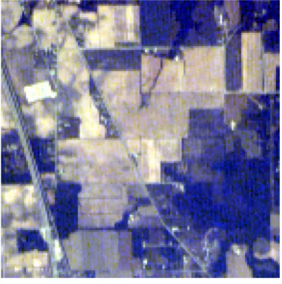
with 220 spectral channels (Figure 2). It is well known due to the complexity of the classification problem it represents. The 16 land use classes consisting mainly of crop classes are to be separated. These are difficult to separate since they are spectrally very similar (due to the early phenological stage of the vegetation).

Although our implementation of Algorithm 2.17 is capable to process 220 features, only the first six principal components are considered. The reason is that there are two sources of coincidences. The first is coincidence due to spectral similarity of land cover classes (signal), the second is coincidence due to noise. For this work, only the coincidence of signal is relevant. Since the algorithm is not fit to distinguish between the two sources, only the six first principal components are considered relevant. They explain 99.66% of the sum of eigenvalues and are therefore believed to contribute considerably to coincidences due to signal and only marginally to coincidence due to noise.

[image:9.595.123.486.270.716.2]

At first, the dataset is classified with a linear kernel SVM as given in Equation (18). A visual result can be seen in Figure 3 (left). The overall accuracy yielded is 53.5% and the

κ

-coefficient is 0.44. As can be seen, the dataset requires more complex kernel functions than linear ones. Then, a multiple kernel K_mult of the form (16) is computed as described in Section 3.1. The dataset is again classified using an SVM, and a visual result can be seen in Figure 3 (right). The overall accuracy yielded is 53.7% and the

κ

-coefficient is 0.45.

Figure 2. Hyperspectral image.

(a) (b)

[image:9.595.197.403.278.486.2]

(10)

The overall accuracy is the percentage of correctly classified pixels from the reference data. The

κ

-coefficient is a statistical measure of the agreement, beyond chance, between the algorithm’s results and the manual labelling in the reference data. Both are global measurements of performance.

As can be seen, both results have a lot of resemblance in the major part. However, the result produced with the linear kernel tends to confuse the brown crop classes in the north with green pasture classes. On the other hand, the linear kernel SVM better recognizes the street in the Western part of the image.

The kernel target alignment between these kernels and the ideal kernel

(

)

ideal i, j L Li, j

K x x =δ

was computed. The ideal kernel is defined via the label L_{associated to each pixel, and has value 1 if the labels} coincide, otherwise its value is zero. Note that the kernel target alignment proposed by [2] represents an a-priori quality assessment of a kernel’s suitability. It is defined as

(

)

ideal

ideal ideal ,

, :

, ,

G

G G

K K A K K

K K K K

=

⋅

where

(

) (

)

, 1

, , ,

n

i j i j G

i j

M N M x x N x x

=

∑

denotes the usual scalar product between Gram matrices.

The kernel target alignment takes values in the interval

[

− +1, 1

]

with one being the best. The kernel target alignment of K_lin was 0.37. The K_mult yielded a higher alignment of 0.47 thus giving reason for expecting a higher overall performance of the latter. The producers’ accuracies

( )

pa and users’ accuracies

( )

ua for the individual classes are shown in Table 1and Table 2.

[image:10.595.92.540.453.724.2]

The users’ accuracy shows what percentage of a particular ground class was correctly classified. The producers’ accuracy is a measure of the reliability of an output map generated from a classification scheme which tells what percentage of a class truly corresponds to a class in the reference. Both are local (i.e. class-dependent) measurements of performance.

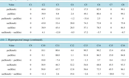
Table 1. Hyperspectral image (channels R:25, G:12, B:1).

Value C1 C2 C3 C4 C5 C6 C7 C8

pa(Kmult) 0 46.6 12.6 1.2 17.5 82.9 0 99.1

pa(Klin) 0 39.9 0.8 2.4 49.1 80.4 0 99.1

pa(Kmult) − pa(Klin) 0 6.7 11.8 −1.2 −31.6 2.5 0 0

ua(Kmult) 0 43.0 33.4 20.0 74.3 72.8 0 75.8

ua(Klin) 0 38.9 45.4 28.5 57.1 78.5 0 84.5

[image:10.595.90.539.459.577.2]

ua(Kmult) − ua(Klin) 0 4.1 −12.0 −8.5 17.2 −5.7 0 −8.7

Table 2. Hyperspectral image (continued).

Value C9 C10 C11 C12 C13 C14 C15 C16

pa(Kmult) 0 10.1 80.6 4.6 90.5 90.2 15.4 63.6

pa(Klin) 0 0.1 88.0 1.1 91.8 86.5 15.0 84.8

pa(Kmult) − pa(Klin) 0 10.0 −7.4 3.5 −1.3 3.7 0.4 −21.2

ua(Kmult) 0 38.9 46.3 32.2 54.0 68.8 45.5 93.3

ua(Klin) 0 50.0 43.7 12.8 56.6 72.5 65.5 86.1

(11)

As had to be expected, each classification approach outperformed the other for some classes. The approach based on K_mult yields higher producers’ accuracy values than K_lin in seven cases. For five cases, K_lin is superior. For users’ accuracy, K_mult is superior in five cases, K_lin in eight cases.

Since producers’ accuracy outlines which amount of pixels from the reference are found in the classification (completeness) while users’ accuracy outlines which amount of the pixels in one class are correct, it can be concluded, that the proposed approach produces more complete results for many classes than with the standard linear kernel approach. Of course, due to the low overall accuracy values yielded, the approach should be ex- tended by applying e.g. Gaussian functions over the similarity matrices.

4. Conclusion

Finding optimal Baire distances defined by permutations of n variables can be done in quadratic time, if the data size is fixed and a gradient descent algorithm is used. For the Baire distance parametrised by the base , this becomes the global minimum if  is sufficiently small. In practice the outcome will be not a unique permutation, but a more or less large set  of optimal permutations σ . The σ can be viewed in a natural way as words over some alphabet. This implies that the symmetric group S_n of the n variables has a well- defined dendrogram D S

( )

_n in which we can view  as a cluster. The common initial word w_ of  defines a ranking of  =

( )

w_ ≤n of the variables which we conjecture to contain the most relevant inherent hierarchical information of the dataset X, after removing variables with very small variation. We expect further hierarchical information about X by finding optimal classifications of  with respect to the ultrametric defined by its dendrogram D

( )

 . Apart from theoretically providing an algorithm which finds the optimal permutation, the applicability of the methodology was demonstrated. To this end, an initial experiment to integrate the Baire distance into state-of-the-art SVM classification is provided. By defining a new multiple kernel function based on Baire distances, classification accuracy on a benchmark dataset is increased. This finding emphasizes the usefulness of the optimal Baire distance in classification. In future work, Gaussian kernels based on the Baire distance will be studied. Furthermore, unsupervised classification algorithms using the permutation-dependent ultrametrics will be dealt with in future work.

Acknowledgements

This work has grown out of a talk given at the International Conference on Classification (ICC 2011) and the discussions afterwards. The first author is funded by Deutsche Forschungsgemeinschaft (DFG), and the second author by the Deutsches Zentrum für Luft-und Raumfahrt e.V. (DLR). Thanks to Fionn Murtagh, Roland Glantz, and Norbert Paul for valuable conversation, as well as Fionn Murtagh and David Wishart for the organising of the International Conference on Classification (ICC 2011) in Saint Andrews, Scotland. The article processing charge was funded by the German Research Foundation (DFG) and the Albert Ludwigs University Freiburg in the funding programme Open Access Publishing.

References

[1] Contreras, P. and Murtagh, F. (2010) Fast Hierarchical Clustering from the Baire Distance. In: Locarek-Junge, H. and Weighs, C., Eds., Classification as a Tool for Research, Springer Berlin Heidelberg, Germany, 235-243.

http://dx.doi.org/10.1007/978-3-642-10745-0_25

[2] Cristianini, N., Shawe-Taylor, J., Elisseeff, A. and Kandola, J. (2006) On Kernel Alignment. In:Holmes, D.E., Ed., Inno-vations in Machine Learning, Springer Berlin Heidelberg, Germany, 205-256.

[3] Murtagh, F. (2004) On Ultrametricity, Data Coding, and Computation. Journal of Classification, 21, 167-184.

http://dx.doi.org/10.1007/s00357-004-0015-y

[4] Benois-Pineau, J., Khrennikov, A.Y. and Kotovich, N.V. (2001) Segmentation of Images in p-Adic and Euclidean Me-trics. Doklady Mathematic, 64, 450-455.

[5] Bradley, P.E. (2010) Mumford Dendrograms. The Computer Journal, 53, 393-404.

http://dx.doi.org/10.1093/comjnl/bxm088

[6] Bradley, P.E. (2008) Degenerating Families of Dendrograms. Journal of Classification, 25, 27-42.

http://dx.doi.org/10.1007/s00357-008-9009-5

(12)

http://dx.doi.org/10.1007/BF00994018

[9] Braun, A.C. (2010) Evaluation of One-Class SVM for Pixe-Based and Segment-Based Classification in Remote Sens-ing. International Archives of Photogrammetry, Remote Sensing and Spatial Information Sciences, 38, 160-165. [10] Braun, A.C., Weidner, U., Jutzi, B. and Hinz, S. (2011) Integrating External Knowledge into SVM Classification—Fus-

ing Hyperspectral and Laserscanning Data by Kernel Composition. In: Heipke, C., Jacobsen, K., Rottensteiner, F., Müller, S. and Sörgel, U., Eds., High-Resolution Earth Imaging for Geospatial Information, International Archives of Photogrammetry, Remote Sensing and Spatial Information Sciences, 38, Part 4/W19 (on CD).

[11] Amari, S. and Wu, S. (1999) Improving Support Vector Machine Classifiers by Modifying Kernel Functions. Neural Networks, 12, 783-789. http://dx.doi.org/10.1016/S0893-6080(99)00032-5

[12] Braun, A.C., Weidner, U., Jutzi, B. and Hinz, S. (2012) Kernel Composition with the One-against-One Cascade for In-tegrating External Knowledge into SVM Classification. Photogrammetrie-Fernerkundung-Geoinformation, 2012, 371- 384. http://dx.doi.org/10.1127/1432-8364/20/0124

[13] Sonnenburg, S., Rätsch, G., Schäfer, C. and Schölkopf, B. (2006) Large Scale Multiple Kernel Learning. The Journal of Machine Learning Research, 7, 1531-1565.