Attractor Based Simultaneous Design of the Minimum Set of Control Nodes and Controllers in Boolean Networks

(1)

http://dx.doi.org/10.4236/am.2016.714131

Attractor-Based Simultaneous Design of

the Minimum Set of Control Nodes and

Controllers in Boolean Networks

Koichi Kobayashi

Graduate School of Information Science and Technology, Hokkaido University, Sapporo, Japan

Received 20 June 2016; accepted 15 August 2016; published 18 August 2016

This work is licensed under the Creative Commons Attribution International License (CC BY).

http://creativecommons.org/licenses/by/4.0/

Abstract

Design of control strategies for gene regulatory networks is a challenging and important topic in systems biology. In this paper, the problem of finding both a minimum set of control nodes (con-trol inputs) and a con(con-troller is studied. A con(con-trol node corresponds to a gene that expression can be controlled. Here, a Boolean network is used as a model of gene regulatory networks, and con-trol specifications on attractors, which represent cell types or states of cells, are imposed. It is im-portant to design a gene regulatory network that has desired attractors and has no undesired at-tractors. Using a matrix-based representation of BNs, this problem can be rewritten as an integer linear programming problem. Finally, the proposed method is demonstrated by a numerical ex-ample on a WNT5A network, which is related to melanoma.

Keywords

Boolean Networks, Integer Linear Programming, Minimum Set of Control Nodes, Singleton Attractors

1. Introduction

(2)

are not necessarily specified, the problem of finding a set of control nodes based on control specifications is important as a kind of inverse problems. Needless to say, it is desirable that the number of control nodes is small.

In this paper, we study simultaneous design of a minimum set of control nodes and controllers in a Boolean networks (BN). A BN [2] is one of the simplified models such as Bayesian networks and piecewise affine sys-tems [3], and is widely used in theoretical analysis of gene regulatory networks (see, e.g., [4]-[19]). In the BN, dynamics such as interactions between genes are expressed by Boolean functions, that is, gene expression is ex-pressed by a binary value (0 or 1). As a generalized version of BNs, a probabilistic BN has been proposed in [20]. In the simultaneous design problem studied in this paper, control specifications on attractors are imposed. Attractors represent cell types or states of cells [21]. In particular, we focus on a singleton attractor, which is al-so called a fixed point. By al-solving this problem, we can obtain a gene regulatory network that has desired at-tractors and has no undesired atat-tractors. Furthermore, we can obtain time evolution (i.e., a Boolean function) of a control node, i.e., a controller by solving this problem. Thus, a solution of the simultaneous design problem provides a helpful suggestion to e.g., design of therapeutic interventions.

As a related problem, the conventional controllability problem of BNs has been widely studied (see, e.g., [7] [12] [13] [17] [18] [22] [23]). However, the problem of finding a minimum set of control nodes has not been considered. In [24], using piecewise affine systems, the problem of choosing a control node has been studied. However, the minimization problem of the number of control nodes has not been considered.

In order to solve the simultaneous design problem, a matrix-based representation of BNs [10] is utilized. Us-ing this representation, this problem can be rewritten as an integer linear programmUs-ing problem. We may use a matrix-based representation using the semi-tensor product (STP) method [7] [25]. Since manipulation of ma-trices using the STP is not needed in this paper, we utilize a simple matrix-based representation using truth tables. The effectiveness of the proposed method is presented by an example on a WNT5A network, which is related to melanoma.

Notation: For the finite set , let  denote the number of elements in . For the n-dimensional vector

[

1 2 n

]

x= x x  x Τ and the index set  =

{

i i1, ,2 ,im

} {

⊆ 1, 2,,n

}

, define

[ ]

xi i : xi1 xi2 xim

Τ ∈ =    . For two matrices A and B, let A⊗B denote the Kronecker product of A and B. In addition, for q vectors

1, 2, , q

y y  y and the index set  =

{

j j1, 2,,jp

}

⊆

{

1, 2,,q

}

, define

⊗

j∈yj:= yj₁⊗yj₂⊗ ⊗ yj_p. For example, for q two-dimensional vectors z z1, 2,,zq and  =

{ }

1, 5 , we can obtain

( ) ( )

( ) ( ) 1 1 1 5

1 2

1 1 5

2 1

5 ₁ ₅

2 2 1 5

= ,

j j

z z

z z z

z

z _z _z

z z

∈

       

=_{ } _ _        

⊗



where z( )ji is the i-th element of zj. Finally, let 1m n× denote the m×n matrix whose elements are all one.

2. Boolean Networks

Consider the following Boolean network (BN):

(

)

(

( )

)

(

)

(

( )

)

(

)

(

( )

)

1

2

1 1

2 2

1 ,

n

j _j

n n j _j

x k f x k

x k f x k

∈

 _{+ =} _ _   



   + =

 _ _

  

 + = _ _ 





(1)

where

[

1 2

]

{ }

0,1

n n

x= x x  x Τ∈ is the state (e.g., the expression of genes), and k∈

{

0,1, 2,

}

is the dis- crete time. The set i⊆

{

1, 2,,n

}

is a given index set, and expresses the adjacency relation of nodes corre- sponding to genes. The function : 0,1

{ }

i

{ }

0,11

i

(3)

or 1.

Next, the notion of attractors is defined as follows.

Definition 1 The state x k

( )

is called asingleton attractor if x k

(

+ =1

)

x k

( )

holds.

Definition 2 The set of states

{

x k

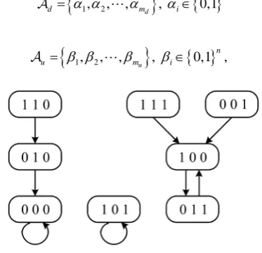
hold. We present a simple example.

Example 1 Consider the following BN:

(

)

( )

(

)

( )

(

)

( )

1 3

2 1 3

3 1 2

1 ,

1 .

x k x k

x k x k x k

x k x k x k

+ = 

 _{+ =} _{∧ ¬} 

 _{+ =} _{∨ ¬} 

(2)

In this BN, ₁=

{ }

3 , ₂=

{ }

1, 3 , and ₃=

{ }

1, 2 hold. Figure 1 shows the state transition diagram.

FromFigure 1, we see that there exist two singleton attractors and one periodic attractor with p=2.  In this paper, we focus on only a set of singleton attractors. Hereafter, let  denote a set of singleton at-tractors for the BN (1).

3. Problem Formulation

The states x x1, 2,,xn are decomposed to two groups xi, i∈ and xi, i∈, where  and  are in-dex sets satisfying  ∪ =

{

1, 2,,n

}

and  ∩ = ∅. Then, defining u k_i

( )

:=x k_i

( )

, i∈, the BN (1) can be rewritten as

(

)

(

( )

)

(

)

(

( )

)

1 , , ,

i i

i i j _j j _j

x k f u k u k i

u k f u k u k i

∈ ∈

 _{+ =} _ _ _ _ _∈

   

 

 + = _ _ _ _ ∈



 





(3)

where i, i, i, and i are an index set. For each i∈ ∪  , the relations i∪ i = i and

i∩ i = ∅

  hold. The Boolean function fi, i∈ is given in advance. The Boolean function fi, i∈ is not given, and must be found. In other words, we consider that some of Boolean functions in the BN (1) are re-placed with new Boolean functions. In the case of = ∅, (3) is the same as (1). Furthermore, in the BN (3),

( )

i

u k corresponds to the control node (i.e., the control input). The Boolean function fi, i∈ can be re-garded as the controller.

Then, consider the following problem.

Problem 1 For the BN (3), suppose that Boolean functions f1,f2,,fn are given. Suppose also that the set

of desired singleton attractors and the set of undesired singleton attractors are given by

{

1, 2, , d

}

,

{ }

0,1 n

d = α α αm αi∈

 (4)

and

{

1, 2, , u

}

,

{ }

0,1 , n

u = β β  βm βi∈

[image:3.595.218.405.517.697.2]

 (5)

Figure 1.State transition diagram, where the number assigned to

(4)

respectively. Then, find a minimum set of control nodes and a controller fi, i∈ satisfying the following two

conditions:

,

d ⊆

  (6)

and

.

u∩ = ∅

  (7) If this problem is infeasible, then there exists no controller that realizes specifications on singleton attractors. This fact implies that the BN (3) is uncontrollable from the viewpoint of singleton attractors, and the change of the graph structure i is required. On the other hand, as a solution, = ∅ may be obtained. This solution implies that a given BN has desired singleton attractors and has no undesired singleton attractors. That is, con-trol nodes are not necessary. Thus, Problem 1 can be regarded as a kind of the concon-trollability problems.

If the set  (i.e., ) is given, Problem 1 has been already solved in [10]. Problem 1 is more general than the problem studied in [10]. By solving Problem 1, we can obtain both the minimum set of control nodes and the controller. To the best of our knowledge, such problem has not been studied so far.

4. Matrix-Based Representation of Boolean Networks

In order to solve Problem 1, we use a matrix-based representation of BNs [10].

( )

1

: i i .

i

i i

x k x k

x k

x k x k

 

   −  = _= _

   

   

Then, the matrix-based representation for x ki

(

+1

)

is given by

(

1 =

)

( )

,

i

i i j

j

x k A x k

∈

+

_⊗



(8)

where Ai

{ }

0,1 2 2 i

×

∈  and

( ) { }

0,12 i

i j

j∈ x k ∈

⊗

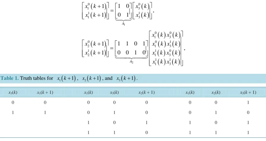
  . The matrix Ai can be derived from truth tables. We present a simple example.

Example 2 Consider the BN (2) again. Then, we can obtain the truth table for each x ki

(

+1

)

. See Table 1.

From these truth tables, we can obtain the following matrix-based representation:

(

)

(

)

( )

1

0 0

1 3

1 1

1 3

1 0 1

, 0 1

1

A

x k x k

x k x k

 +    

=

 ₊    

    

  _ 

(

)

(

)

( ) ( )

2

0 0

1 3

0 0 1

2 1 3

1 1 0

2 1 3

1 1

1 3

1 1 0 1

1

,

0 0 1 0

1

A

x k x k

x k x k x k

x k x k x k

x k x k

 

 

 + ₌ _{ } _

 ₊   _{ } _

   

  _ _

 

 

[image:4.595.86.537.488.727.2]



.

x3(k) x1(k + 1) x1(k) x3(k) x2(k + 1) x1(k) x2(k) x3(k + 1)

0 0 0 0 0 0 0 1

1 1 0 1 0 0 1 0

1 0 1 1 0 1

(5)

(

)

(

)

( ) ( )

3

0 0

1 2

0 0 1

3 1 2

1 1 0

3 1 2

1 1

1 2

0 1 0 0

1

,

1 0 1 1

1

A

x k x k

x k x k x k

x k x k x k

x k x k

 

 

 + ₌ _{ } _

 ₊   _{ } _

   

  _ _

 

 



where each element of Ai, i=1, 2, 3 is given by a binary value (0 or 1), and a sum of all elements in each

column of Ai is equal to 1. The second row in Ai, i=1, 2, 3 corresponds to the column in x ki

(

+1

)

in truth

tables. 

See [10] for further details of deriving the matrix Ai.

The matrix-based representation is useful for considering Problem 1. Using the matrix-based representation, the problem of finding a Boolean function is reduced to the problem of finding Ai. The latter problem is rela-tively easier than the former problem, and can be solved by using some computational tools.

Remark 1 Recently, there have been many results about a matrix-based representation of Boolean functions using the semi-tensor product (STP) of matrices (see, e.g., [7] [25]). Of course, the matrix-based representation using the STP method may be utilized. In this paper, we focus on singleton attractors (i.e., the steady state), and time sequences of the state are not computed. Hence, manipulation of matrices using the STP is not needed, and the simple matrix-based representation using truth tables is utilized.

5. Solution Method for Problem 1

Based on the matrix-based representation of BNs explained in the previous section, we consider a solution me-thod for Problem 1.

As preparations, the notation is defined. If Ai in (8) includes decision variables, then Ai is denoted by Ai. Let αi( )j and

( )j i

β denote the j-th element of αi and βi in d of (4) and u of (5), respectively. De- fine

( ) ( )

( )

( ) ( )

( )

1 1

: , : .

j j

j i j i

i _j i _j

i i

α β

 −   − 

=  = 

   

   

Since only singleton attractors are focused in Problem 1, Problem 1 is equivalently transformed into the fol-lowing problem.

Problem 2 Find matrices A A 1, 2,,An and binary variables δ δ1, 2,,δn minimizing the cost function

1

n i i=δ

∑

subject to the following two conditions. (i) For each i∈

{

1, 2,,md

}

, the following constraints

}

( )

1

2

1

1 1 1 1

2

2 2 2 2

1 ,

1 .

n

j

i i

j

i i

j

n j

i n n n n i

j

A A

α δ δ α

∈

= − +

⊗









(ii) For each i∈

{

1, 2,,m_u

₎

}

( )

1

2

1

1 1 1 1

2

2 2 2 2

1 ,

1 .

n

j

i i

j

i i

j

n j

i n n n n i

j

A A

β δ δ β

∈

≠ − +

⊗









(6)

is equal to 1. 

In this problem, the condition (i) guarantees that x k

(

+ =1

)

x k

( )

=αi, i=1, 2,,md , that is, αi,

1, 2, , _d

i=  m are included in the set of singleton attractors. The condition (ii) guarantees that βi, i=1, 2,,md are not a singleton attractor. If δ_i =0, i=1, 2,,n are obtained as a solution, then this solution implies

= ∅

 , that is, the controller is not needed. If δ_i =1, i=1, 2,,n are obtained as a solution, then this solution implies = ∅, that is, all Boolean functions are changed.

Problem 2 can be rewritten as an integer linear programming (ILP) problem, and can be solved by a suitable solver. An SMT (Satisfiability Modulo Theories) solver such as the Yices SMT Solver [26] can also be applied to Problem 2.

Here, using a simple example, we explain a method to rewrite Problem 2 as an ILP problem. Consider the BN in Example 2 of Section 4. Then, the constraints appeared in Problem 2 are given by

( )

(

)

( )

1 2

1 11 12 1

1 1

1 2

11 12

1 1

1 0 1 1 1 1

1 , 1 0 a a a a α α δ δ α α  − ₌ ₋  ₊  − −  −                   

    (9)

( )

(

)

( )

2 1

1 21 22 1

2 2

2 1

21 22

1 1

1 1 0 1 1 1

1 , 0 1 a a a a α α δ δ α α  ₋  __ _ _ _ ₋ ₋ __{ −}_  = − +   _    _              (10) ( ) ( )

(

)

( )

(

)

(

( )

)

( )

(

)

( ) ( )

(

( )

)

( ) ( )

( )1 ( )2 1 1 1 2 1 1 1 2 3 1 1

31 32 33 34

1

3 3

3

1 2

31 32 33 34

1 1 1 1 2 1 1 1 1 1

1 1 1 1

1 1 1 0 1

1

0 0 1 0

1

a a a a

α α

α α α

δ δ

α _α _α

α α ⊗  ₋ ₋       − ₌ ₋  ₊  − − − −   −        _ _             −         (11) and ( ) ( )

(

)

( ) ( ) 1 2

1 11 12 1

1 1

1 2

11 12

1 1

1 0 1 1 1 1

1 , 1 0 a a a a β β δ δ β β  ₋  __ _ _ _ ₋ ₋ __{ −}_  ≠ − +   _    _              (12) ( ) ( )

(

)

( ) ( ) 2 1

1 21 22 1

2 2

2 1

21 22

1 1

1 1 0 1 1 1

1 , 0 1 a a a a β β δ δ β β  − _≠ ₋  ₊  − −  −                   

    (13)

( ) ( )

(

)

( )

(

)

(

( )

)

( )

(

)

( ) ( )

(

( )

)

( ) ( )

( )1 ( )2 1 1 1 2 1 1 1 2 3 1 1

31 32 33 34

1

3 3

3 ₁ ₂

31 32 33 34

1 1 1 1 2 1 1 1 1 1

1 1 1 1

1 1 1 0 1

1 ,

0 0 1 0

1

a a a a

β β

β β β

δ δ

β _β _β

β β ⊗  ₋ ₋       − _≠ ₋  ₊  − − − −   −        _ _             −        

where aij is a binary decision variable. From (9)-(11), we can obtain

( )

2 1 ( )1 ( )2

1 1 11 1 1

1 12 1 1 0

1,

0 0 1 a

a

δ

α δ α α

δ

Τ−   

 = + −  _{ } _  _{ } _   (14) ( )

( )

1 2 ( )2 ( )1

1 2 21 1 1

2 22

0 1 0

,

1 0 1 a

a

δ

α δ α α

δ

Τ   

 = − ₋ _{ } _  _{ } _  

(7)

( ) ( )

(

)

( ) ( )

(

( )

)

3

3 31

1 2 3 1 2

1 1 3 32 1 1 1

3 33

3 34

0 1 0 0 0

0 0 1 0 0

1 .

1 0 0 1 0

0 0 0 0 1

a a a a δ δ

α α δ α α α

δ δ Τ    _{ }   _{ } _  _{ } _ ⊗ = − − −    _{ }   _{ } _   (16)

From (12)-(14), we can obtain

( )

2 1 ( )1 ( )2

1 1 11 1 1

1 12

1 1 0

1,

0 0 1 a

a

δ

β δ β β

δ

Τ−   

 ≠ + −  _{ } _  _{ } _   (17) ( )

( )

1 2 ( )2 ( )1

1 2 21 1 1

2 22

0 1 0

,

1 0 1 a

a

δ

β δ β β

δ

Τ   

 ≠ − ₋ _{ } _  _{ } _   (18) ( ) ( )

(

)

( ) ( )

(

( )

)

3 3 31

1 2 3 1 2

1 1 3 32 1 1 1

3 33

3 34

0 1 0 0 0

0 0 1 0 0

1 .

1 0 0 1 0

0 0 0 0 1

a a a a δ δ

β β δ β β β

δ δ Τ    _{ } _  _{ } _  _{ }  ⊗ ≠ − − −    _{ } _  _{ } _   (19)

From the condition (ii) in Problem 2, at least one of (17)-(19) must be satisfied. Noting this fact, from (17)-(19) we can obtain

( )

2 1 ( )1 ( )2

1 1 11 1 1 1,1 1,2

1 12 1 1 0

1 ,

0 0 1 a

a

δ

β δ β β δ δ

δ

Τ−   

 + − − = −  _{ } _  _{ } _   (20) ( )

( )

1 2 ( )2 ( )1

1 2 21 1 1 2,1 2,2

2 22

0 1 0

,

1 0 1 a

a

δ

β δ β β δ δ

δ

Τ   

 − + = − ₋ _{ } _  _{ } _   (21) ( ) ( )

(

)

( ) ( )

(

( )

)

3 3 31

1 2 3 1 2

1 1 3 32 1 1 1 3,1 3,2

3 33

3 34

0 1 0 0 0

0 0 1 0 0

1 ,

1 0 0 1 0

0 0 0 0 1

a a a a δ δ

β β δ β β β δ δ

δ δ Τ    _{ } _  _{ }   _{ } _ ⊗ − + − = − −    _{ } _  _{ } _   (22)

where δi,1, δi,2, i=1, 2, 3 are additional binary variables satisfying the two constraint conditions 3

,1 ,2 ,1 ,2

1

1, 1.

i i i i

i

δ δ δ δ

=

+ ≤

∑

+ ≥ (23)

Under these conditions, at least one of δi,1−δi,2, i=1, 2, 3 takes either −1 or 1. Thus, Problem 2 for the BN in Example 2 can be rewritten as the following problem.

11 12 21 22 31 32 33 34 1 2 3 ,1 ,2

1 2 3

find , , , , , , , , , , , , , 1, 2, 3,

min ,

i i

a a a a a a a a δ δ δ δ δ i

δ δ δ

= + +

subject to (14)-(16), (20)-(22), and (23).

Finally, the product of binary variables such as δ1 11a can be linearized by using the following lemma [27].

(8)

j j

z=

∏

_∈_δ is equivalent to the following linear inequalities

1, 0,

j j

z z

δ δ

∈ ∈

− ≤ − − + ≤

∑

 

where  is the cardinality of .

Using this lemma, Problem 2 for the BN in Example 2 can be rewritten as an ILP problem. From the above, we see that Problem 2 for a general BN (3) can be rewritten as an ILP problem. In general, an ILP problem is NP-hard, but several free/commercial solvers were developed. Hence, we can solve the ILP problem obtained.

6. Example on a WNT5A Network

In this section, as an example, we consider the gene regulatory network with the gene WNT5A, which is related to melanoma. A BN model is given by

(

)

( )

1 1 6 ,

x k+ = ¬x k

(

)

(

( )

)

{

( )

(

where the concentration level (high or low) of the gene WNT5A is denoted by x1, the concentration level of the gene pirin by x2, the concentration level of the gene S100P by x3, the concentration level of the gene RET1 by x4, the concentration level of the gene MART1 by x5, the concentration level of the gene HADHB by x6, and the concentration level of the gene STC2 by x7. See [28] for further details.

For this BN model, consider solving Problem 1. We assume that d, and u are given by

[

]

{

0 0 0 0 0 1 1

}

,

d

Τ

= 

[

]

{

1 1 0 1 1 1 1

}

,

u

Τ

= 

respectively. This setting is artificially given.

First, we derive a matrix-based representation. Then, we can obtain the following matrix-based representa-tion:

(

)

(

)

( )

0 0

1 6

1 1

1 6

0 1 1

,

1 0

1

x k x k

x k x k

 + ₌    ₊         

   

(

)

(

)

( ) ( ) ( )

2 4 6

0 0 0

2 4 6

0 0 1

2 4 6

0 1 0

2 4 6

0 0 1 1

2 2 4 6

1 1 0 0

2 2 4 6

1 0 1

2 4 6

1 1 0

2 4 6

1 1 1

2 4 6

1 1 1 0 1 0 0 0

1

,

0 0 0 1 0 1 1 1

1

x k x k x k

x k x k x k

x k x k x k x k

x k x k x k

⊗ ⊗

 

 

 + ₌   

 ₊     

   

  _ _

 

 

(9)

(

)

(

)

( )

0 0

3 7

1 1

3 7

0 1 1

,

1 0

1

x k x k

x k x k

 + ₌    ₊         

   

(

)

(

)

( )

0 0

4 4

1 1

4 4

1 0

1

, 0 1

1

x k x k

 + ₌    ₊         

   

(

)

(

)

( ) ( )

2 7

0 0

2 7

0 0 1

5 2 7

1 1 0

5 2 7

1 1

2 7

0 1 0 0

1

,

1 0 1 1

1

x k x k

x k x k

x k x k x k

x k x k x k

x k x k

⊗

 

 

 + ₌ _{ } _

 ₊   _{ } _

   

  _ _

 

 



(

)

(

)

( ) ( )

3 4

0 0

3 4

0 0 1

6 3 4

1 1 0

6 3 4

1 1

3 4

1 0 0 0

1

,

0 1 1 1

1

x k x k

x k x k

x k x k x k

x k x k x k

x k x k

⊗

 

 

 +   _{ } _

=

 ₊   _{ } _

   

  _ _

 

 



(

)

(

)

( ) ( )

2 7

0 0

2 7

0 0 1

7 2 7

1 1 0

7 2 7

1 1

2 7

0 0 1 0

1

.

1 1 0 1

1

x k x k

x k x k

x k x k x k

x k x k

⊗

 

 

 + ₌ _{ } _

 ₊   _{ } _

   

  _ _

 

 



Next, we explain the solution for Problem 2. By solving this problem, we can obtain δ6=1 and δi =0,

1, 2, 3, 4, 5, 7

i= . That is, the minimum value of  is obtained by 1, and the sets  and  are obtained by

{

1, 2, 3, 4, 5, 7

}

=

 and =

{ }

6 , respectively. This implies that only the Boolean function

(

)

( )

6 1 3 4

x k+ =x k ∨x k must be replaced with other Boolean function. As the solution, we can obtain

(

)

( )

6 1 3 4 .

x k+ =x k ∨ ¬x k

Finally, we observe the set of singleton attractors. For the BN model obtained, the set of singleton attractors is given by

[

] [

]

{

[

] [

]

}

0 0 0 0 0 1 1 , 0 1 0 0 1 1 1 , 0 1 1 0 1 1 0 ,

1 0 0 1 0 0 1 , 1 1 0 1 1 0 1 .

Τ Τ Τ

Τ Τ

= 

From this set, we see that specifications on singleton attractors (d ⊆ of (6) and u∩= ∅ of (7)) are satisfied.

7. Conclusions

For Boolean networks, we studied the problem of finding both a minimum set of control nodes and a controller, where specifications on singleton attractors are imposed. In biological networks, control nodes (control input) are not necessarily given. Hence, this problem is important in both systems biology and synthetic biology. Using a matrix-based representation of BNs, this problem can be rewritten as an integer linear programming problem. The proposed method is effective as one of the fundamental methods for control theory of gene regulatory networks.

(10)

proposed method, it is important to consider applying the proposed method to several biological systems.

Acknowledgements

This research was partly supported by JSPS Grant-in-Aid for Scientific Research (C) 26420412.

References

[1] Santos-Rosa H. and Caldas, C. (2005) Chromatin Modifier Enzymes, the Histone Code and Cancer. European Journal of Cancer, 41, 2381-2402. http://dx.doi.org/10.1016/j.ejca.2005.08.010

[2] Kauffman, S.A. (1969) Metabolic Stability and Epigenesis in Randomly Constructed Genetic Nets. Journal of Theo-retical Biology, 22, 437-467. http://dx.doi.org/10.1016/0022-5193(69)90015-0

[3] Jong, H.D. (2002) Modeling and Simulation of Genetic Regulatory Systems: A Literature Review. Journal of Compu-tational Biology, 9, 67-103. http://dx.doi.org/10.1089/10665270252833208

[4] Akutsu, T., Hayashida, M., Ching, W.-K. and Ng, M.K. (2007) Control of Boolean Networks: Hardness Results and Algorithms for Tree Structured Networks. Journal of Theoretical Biology, 244, 670-679.

http://dx.doi.org/10.1016/j.jtbi.2006.09.023

[5] Azuma, S., Yoshida, T. and Sugie, T. (2014) Structural Monostability of Activation-Inhibition Boolean Networks.

Proceedings of the 53rd IEEE Conference on Decision and Control, Los Angeles, 15-17 December 2014, 1521-1526.

http://dx.doi.org/10.1109/CDC.2014.7039615

[6] Chaves, M. (2009) Methods for Qualitative Analysis of Genetic Networks. Proceedings of the European Control Con-ference, Budapest, 23-26 August 2009, 671-676.

[7] Cheng, D. and Qi, H. (2009) Controllability and Observability of Boolean Control Network. Automatica, 45, 1659- 1667. http://dx.doi.org/10.1016/j.automatica.2009.03.006

[8] Kobayashi, K., Imura, J. and Hiraishi, K. (2010) Polynomial-Time Algorithm for Controllability Test of a Class of Boolean Biological Networks. EURASIP Journal on Bioinformatics and Systems Biology, 2010, Article ID: 210685. [9] Kobayashi, K. and Hiraishi, K. (2013) Optimal Control of Gene Regulatory Networks with Effectiveness of Multiple

Drugs: A Boolean Network Approach. BioMed Research International, 2013, Article ID: 246761.

[10] Kobayashi, K. and Hiraishi, K. (2014) ILP/SMT-Based Method for Design of Boolean Networks Based on Singleton Attractors. IEEE/ACM Transactions on Computational Biology and Bioinformatics, 11, 1253-1259.

[11] Langmead, C.J. and Jha, S.K. (2009) Symbolic Approaches to Finding Control Strategies in Boolean Networks. Jour-nal of Bioinformatics and ComputatioJour-nal Biology, 7, 323-338. http://dx.doi.org/10.1142/S0219720009004084

[12] Laschov, D. and Margaliot, M. (2009) Controllability of Boolean Control Networks via the Perron-Frobenius Theory.

Automatica, 48, 1218-1223. http://dx.doi.org/10.1016/j.automatica.2012.03.022

[13] Li, F. and Sun, J. (2012) Controllability of Higher Order Boolean Control Networks. Applied Mathematics and Com-putation, 219, 158-169. http://dx.doi.org/10.1016/j.amc.2012.05.059

[14] Li, H., Wang, Y. and Xie, L. (2015) Output Tracking Control of Boolean Control Networks via State Feedback: Con-stant Reference Signal Case. Automatica, 59, 54-59. http://dx.doi.org/10.1016/j.automatica.2015.06.004

[15] Li, F. (2016) Pinning Control Design for the Stabilization of Boolean Networks. IEEE Transactions on Neural Net-works and Learning Systems, 27, 1585-1590. http://dx.doi.org/10.1109/TNNLS.2015.2449274

[16] Li, H., Xie, L. and Wang, Y. (2016) On Robust Control Invariance of Boolean Control Networks. Automatica, 68, 392-396. http://dx.doi.org/10.1016/j.automatica.2016.01.075

[17] Lu, J., Zhong, J., Huang, C. and Cao, J. (2016) On Pinning Controllability of Boolean Control Networks. IEEE Trans-actions on Automatic Control, 61, 1658-1663. http://dx.doi.org/10.1109/TAC.2015.2478123

[18] Srihari, S., Raman, V., Leong, H.W. and Ragan, M.A. (2014) Evolution and Controllability of Cancer Networks: A Boolean Perspective. IEEE/ACM Transactions on Computational Biology and Bioinformatics, 11, 83-94.

http://dx.doi.org/10.1109/TCBB.2013.128

[19] Tournier, L. and Chaves, M. (2009) Uncovering Operational Interactions in Genetic Networks Using Asynchronous Boolean Dynamics. Journal of Theoretical Biology, 260, 196-209. http://dx.doi.org/10.1016/j.jtbi.2009.06.006

[20] Shmulevich, I., Dougherty, E.R., Kim, S. and Zhang, W. (2002) Probabilistic Boolean Networks: A Rule-Based Un-certainty Model for Gene Regulatory Networks. Bioinformatics, 18, 261-274.

http://dx.doi.org/10.1093/bioinformatics/18.2.261

(11)

[22] Li, H. and Wang, Y. (2012) On Reachability and Controllability of Switched Boolean Control Networks. Automatica,

48, 2917-2922. http://dx.doi.org/10.1016/j.automatica.2012.08.029

[23] Zhang, L. and Zhang, K. (2013) Controllability and Observability of Boolean Control Networks with Time-Variant Delays in States. IEEE Transactions on Neural Networks and Learning Systems, 24, 1478-1484.

http://dx.doi.org/10.1109/TNNLS.2013.2246187

[24] Azuma, S., Yanagisawa, E. and Imura, J. (2008) Controllability Analysis of Biosystems Based on Piecewise Affine Systems Approach. IEEE Transactions on Automatic Control, 53, 139-152.

http://dx.doi.org/10.1109/TAC.2007.911316

[25] Cheng, D., Qi, H. and Li, Z. (2011) Analysis and Control of Boolean Network: A Semi-Tensor Product Approach. Springer, Berlin. http://dx.doi.org/10.1007/978-0-85729-097-7

[26] Yices SMT Solver. http://yices.csl.sri.com/

[27] Cavalier, T.M., Pardalos, P.M. and Soyster, A.L. (1990) Modeling and Integer Programming Techniques Applied to Propositional Calculus. Computers & Operations Research, 17, 561-570.

http://dx.doi.org/10.1016/0305-0548(90)90062-C

[28] Xiao, Y. and Dougherty, E.R. (2007) The Impact of Function Perturbations in Boolean Networks. Bioinformatics, 23, 1265-1273. http://dx.doi.org/10.1093/bioinformatics/btm093

Submit or recommend next manuscript to SCIRP and we will provide best service for you:

Accepting pre-submission inquiries through Email, Facebook, LinkedIn, Twitter, etc. A wide selection of journals (inclusive of 9 subjects, more than 200 journals) Providing 24-hour high-quality service

User-friendly online submission system Fair and swift peer-review system

Efficient typesetting and proofreading procedure

Display of the result of downloads and visits, as well as the number of cited articles Maximum dissemination of your research work