http://dx.doi.org/10.4236/ojmsi.2016.42007
How to cite this paper: Gustafsson, L. and Sternad, M. (2016) A Guide to Population Modelling for Simulation. Open Journal of Modelling and Simulation, 4, 55-92. http://dx.doi.org/10.4236/ojmsi.2016.42007
A Guide to Population Modelling for
Simulation
Leif Gustafsson, Mikael Sternad
Signals and Systems, Department of Engineering and Sciences, Uppsala University, Uppsala, Sweden
Received 24 March 2016; accepted 24 April 2016; published 27 April 2016
Copyright © 2016 by authors and Scientific Research Publishing Inc.
This work is licensed under the Creative Commons Attribution International License (CC BY). http://creativecommons.org/licenses/by/4.0/
Abstract
This paper outlines the fundamentals of a consistent theory of numerical modelling of a popula-tion system under study. The focus is on the systematic work to construct an executable simula-tion model. There are six fundamental choices of model category and model constituents to make. These choices have a profound impact on how the model is structured, what can be studied, possi-ble introduction of bias, lucidity and comprehensibility, size, expandability, performance of the model, required information about the system studied and its range of validity. The first choice concerns a discrete versus a continuous description of the population system under study—a choice that leads to different model categories. The second choice is the model representation (based on agents, entities, compartments or situations) used to describe the properties and be-haviours of the objects in the studied population. Third, incomplete information about structure, transitions, signals, initial conditions or parameter values in the system under study must be ad-dressed by alternative structures and statistical means. Fourth, the purpose of the study must be explicitly formulated in terms of the quantities used in the model. Fifth, irrespective of the choice of representation, there are three possible types of time handling: Event Scheduling, Time Slicing or Micro Time Slicing. Sixth, start and termination criteria for the simulation must be stated. The termination can be at a fixed end time or determined by a logical condition. Population models can thereby be classified within a unified framework, and population models of one type can be trans-lated into another type in a consistent way. Understanding the pros and cons for different choices of model category, representation, time handling etc. will help the modeller to select the most ap-propriate type of model for a given purpose and population system under study. By understanding the rules for consistent population modelling, an appropriate model can be created in a systematic way and a number of pitfalls can be avoided.
Keywords
56
1. Introduction
Understanding is based on models. Modelling is a way to describe a part of the universe—denoted the system under study—by creating a model, or theory, that is useful for a given purpose. The intention behind all types of models (mental, physical, analogous, mathematical or numerical) is to provide a very simplified description of important aspects of a system under study. The principle of parsimony, also denoted Occam’s razor, can be phrased as: “A scientific theory [model] should be as simple as possible, but no simpler.” (A. Einstein). This al-so means that “there are no true models—but al-some are useful” (G. Box).
In this paper, we confine our attention to the field of population models that are intended to be used for simu-lation. A population model is a type of model that is applied to the study of population dynamics. Central in such models are the concepts of births and deaths, which may include creation, immigration, emigration, de-struction etc. For the mathematical theory of deterministic and stochastic population models, see e.g. [1].
Here we use the word population in a wide meaning, including not only individual humans or animals, but also e.g. cars in traffic or production of items, perhaps in a queuing situation. For example, a model of a farm with a few workers, two tractors, a harvester and some trailers can be regarded as a population model. Popula-tion models are common in many fields such as demography, ecology, epidemiology, traffic studies and manu-facturing, where queues are an important aspect, and also in physics and chemistry.
Using numerical methods, considerably more complex models can be constructed and studied than is possible with only mathematical and statistical methods. Moreover, when no analytical solution can be obtained, the nu-merical approach makes it possible to stepwise update (simulate) the model’s behaviour over time and space.
A general methodology for model building and simulation has been developed, accepted and used for more than half a century. It prescribes that the model study be organised as a project containing a well-defined se-quence of consecutive phases. Apart from terminology, which varies somewhat, a model study should contain the following sequence of project phases: problem definition, model building, validation of model, analysis
based on the validated model, result evaluation and result presentation [2]-[6]. It is also stressed that this process is highly iterative, because learning occurs during the process and makes it necessary to go back and re-fine the model.
The content and methods of each phase are well defined, except for the model building phase. For population studies, there are a number of quite different modelling approaches—based on different ideas and concepts— that can be used. The main classical approaches are outlined in Section 1.2. These approaches have their pros and cons for different purposes and population systems under study. They may produce different results and conclu-sions unless some crucial rules, which are presented in this paper, are strictly followed. This lack of scientifical-ly based general rules for the model building phase has often led to unmotivated approaches or ad hoc construc-tions of the model. Therefore, modelling and simulation are often regarded as a mixture of art and science.
1.1. The Aim of This Paper
The aim of this paper is to complement the science on the model building phase for population models by clari-fying the fundamental constituents of a numerical model of populations under study, and to show how a unified theory of population models can be based on these constituents. It is also our explicit aim to present the paper as a tutorial.
To avoid confusion, it was necessary to find unambiguous terms that work for all types of population models. For example, the term “state”, which has different meanings for different types of model, usually has to be avoided. It was also necessary to introduce and rename some terms.
Furthermore, it was necessary to clearly separate the concepts of the system under study from those of the model world. We observe the objects in the system under study and describe them as subjects that can act in a simulation model. Therefore, the following convention is used throughout: The system under study, containing a
population of objects, is described by a set of subjects in the model.
Depending on the purpose, the modeller is free to model each object as a separate subject, to aggregate sub-jects into different compartments or even to describe the population as a continuous substance, provided that this does not introduce misleading results.
Within this scope of this paper we discuss a number of central issues, such as:
How can a conceptual model be constructed, from the purpose(s) and the system under study?
57
When and how can different types of models be translated into another type?
When will a discrete model and a continuous model give consistent results?
What factors of the population system under study and the problem definition should cause the modeller to choose or avoid specific types of models?
How does the type of model affect the study in terms of required information, size of the model and possibil-ity to include different types of stochasticpossibil-ity?
Note that this paper is not about how to perform a complete modelling study over the sequence of project phases and the iterations involved, nor is it about specific simulation languages or various techniques such as parameter estimation, integration methods, validation or statistical post-processing over many replications. The focus is instead on the “anatomy” of the model, i.e. the main constituent elements and their interrelations, the options available and the consequences of selecting one rather than another of these options.
1.2. Modelling Paradigms and Tools
In this section we briefly introduce some of the classical types of models that exist, roughly in the order in which they were first proposed.
While mental modelling and mental simulation certainly go back to prehistoric times, scientific modelling based on e.g. physical properties of the system under study and expressed in mathematical terms has developed gradually in an ad hoc manner, to handle different issues, during the past few centuries.
A significant milestone is dynamic modelling, which goes back to Isaac Newton [7]. A system of ordinary differential equations is then solved over time, so that the dynamics generated by a physical structure can be re-vealed in the form of e.g. trajectories over time. In this paper we classify this as deterministic compartment- based modelling. A Continuous System Simulation Language may be used for simulating such models.
With the introduction of Monte Carlo methods/simulation in the Manhattan project, the stochastic part of si-mulation started to develop significantly. The idea behind Monte Carlo sisi-mulation is to perform repeated ran-dom experiments to obtain numerical estimates of an unknown quantity. This idea was first proposed by Georges Louis Leclerc, Comte de Buffon, in the paper Sur le jeu de franc-carreau, published in 1777. Monte Carlo methods are mainly used for optimisation, numerical integration and generating draws from a probability distribution. The development of random number generators for different distributions is an important heritage included in most types of simulation packages.
In 1906, Markov chain models were developed as a mathematical/statistical theory of stochastic processes [8] [9]. Later, the development of digital computers made this approach more practically useful. We classify this as
situation-based modelling in our vocabulary.
With digital computers, numerical methods and various kinds of simulation languages, the number of model-ling and simulation approaches virtually exploded during the second half of the 20th century.
In 1961, the entity-based simulation language GPSS was constructed by Geoffrey Gordon [10]. In GPSS, the objects are represented by entities (sometimes called transactions) with identity and attributes (called parameters) that move in a flowchart, which connects various types of stations (called blocks). For these languages, a large number of random number generators for different statistical distributions are included. A drawback with enti-ty-based simulation models is that the number of modelling primitives (station blocks and transport facilities) becomes very large, but still without covering all possibilities.
With SIMULA (1967), the concept of classes of subjects (called “objects”) containing both attributes and procedures was introduced [11]. This opened the way for agent-based simulation. Originally, simulation in SIMULA was performed by the built-in “Class Simulation”. Later on, the powerful “Class DEMOS” [12] could be used for efficient agent-based modelling. The number of concepts and constructions could then be reduced to a small number, leaving details to be specified in the host language SIMULA—an “object-oriented” general- purpose programming language.
58
1.3. Some Previous Work on Unifying Frameworks
There have been a number of attempts to systemise simulation models, to investigate consistency for models in different representations or to compare the merits of different types of simulation models.
In the book “System Simulation: Programming Styles and Languages” [4], simulation is classified by Kreutz-er into four paradigms: “Monte-Carlo methods, continuous, discrete event and combined simulation all have their own methodologies, tools, traditions, user communities and prototypical applications.” The four paradigms are not compared, but presented and discussed side by side.
The book “Theory of Modelling and Simulation: Integrating Discrete Event and Continuous Complex Dy-namic Systems” by Zeigler et al. [15] uses a systems theory approach based on mathematical set theory and fuzzy sets (for handling stochasticities) “for integrating the continuous and discrete paradigms for modelling and simulation”. This provides an impressive but abstract mathematical theory where the system under study, pur-pose and technical modelling details are not in the foreground.
In addition, a large number of papers compare or discuss (stochastic) individual-based models versus analyti-cal models (differential or difference equation models) in a deterministic or stochastic setting, primarily within ecology; see e.g. [16]-[21]. In some of these papers the analytical model is regarded as the base for theory building and becomes a norm (instead of using the system under study as the norm, which we do in this paper). Discrepancies are often found because the assumed analytical model is deterministic or includes stochasticity simply as additive noise. However, we now know the correct ways of introducing different types of stochastici-ties into analytical models, which are presented and used in this paper. We have also recently clarified condi-tions for deterministic and stochastic analytical models to be consistent [22].
In this paper we take a pragmatic approach, focusing on the “anatomical” aspect of what constituents are ne-cessary to model a population system under study. Based on earlier studies [13] [14] [22]-[24], the issues of con- sistency, how to translate between different model representations and pros and cons of choosing a specific re-presentation are covered. The main issue is how well a population system under study can be conceptualised in-to a general conceptual model, and then realised in various ways.
1.4. Outline of the Main Concepts
A common mistake by modellers and readers of simulation-based studies is confusing real system and model. When performing population modelling to be used for simulation, we deal with a system under study, a concep-tual model description of this system and a realisation in the form of an executable numerical model, in the fol-lowing denoted a simulation model. To distinguish between these contexts as clearly as possible, we introduce the picture of different “worlds” in which the system under study, the conceptual model and possible alternative simulation models of it reside.
The SYSTEMS WORLD contains the system under study as an actual, historical, future, assumed or possi-ble reality.
The CONCEPTUAL WORLD is an intermediate world where the purpose of the study and the main com-ponents of the system under study are specified in terms of a conceptual model. Here the focus is on what to model.
The SIMULATION MODELS WORLD is where a simulation model is created from the conceptual model, in order to behave in (almost) the same way as the system under study from the point of view defined by the purpose of the study. The simulation model can then be used for calculations and experiments. Here the fo-cus is on how to model it.
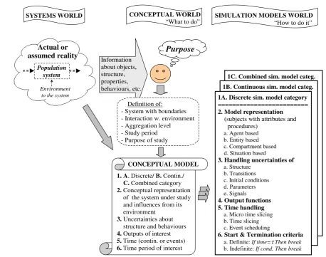
Modelling a system under study for a given purpose is a stepwise procedure, moving from selected proper-ties of the systems world via the conceptual world to the simulation models world where we construct a si-mulation model. An “anatomical” sketch of the main elements and how they are translated between the dif-ferent worlds is provided inFigure 1. The figure also gives an outline of the organisation and content of this paper.
59
Figure 1. An “anatomical” sketch of the construction elements in modelling a population system. Left: The systems world. Centre) The conceptual world. Right: The simulation models world. Note that the purpose and the system under study are both required when specifying the conceptual model. These and other characteristics also affect the realisation of a simula-tion model. This figure defines six main constituents of a simulasimula-tion model that have to be conceptualised and realised.
De-tails of the figure are explained in the following chapters.
2. The Systems World
The universe as we know it is immensely huge and complex, with some 1080 atoms forming various hierarchies of interacting parts. In different sciences and other contexts, different parts of the universe are studied at differ-ent aggregation levels and with differdiffer-ent purposes. The system to be studied may be an actual part of reality, but it may also be an historical or a future situation or an assumed or possible reality.
Before we define/select a specific system in the next chapter, here we only talk about a system in generic terms. Mathematically, a system is a defined subset of components and relations between these components. By focusing on a system under study, we imagine the universe to be divided into two parts: The system under study
andits environment. Abstractly, we think of this in terms of boundaries around the system. These boundaries can be geographical, but they can also frame the types of objects to consider, and define the level of detail to focus on when later describing their properties and behaviours. Thus, the definition of a system is entirely a mental construction that comes from an ambition to focus on a part of the universe at an appropriate level of detail.
60
Furthermore, the boundaries between the system under study and its environment are generally not closed. Even with carefully defined system boundaries, there is usually some form of interchange of material, energy or information between the system and its environment that may also have to be considered. There may be inflows
and outflows of objects through the system boundaries, and the environment may influence the system’s beha-viour.
Since population modelling is of interest here, the system under study will contain a population of discrete objects. These objects can also have a number of properties and behaviours. For example, objects can have the
properties age, sex, position etc. and behaviour that can be to approach, avoid or react to a certain situation. All the above-mentioned aspects are necessary to consider in the subsequent modelling of a particular system, where the system under study can be regarded as a database of more and less relevant information. This is treated in the following chapters.
3. The Conceptual Model (What to Model)
3.1. Introduction
A model study usually starts after some kind of problem recognition—something is interesting, behaves in a strange way, does not work well, could perhaps function in a different way etc. Therefore, the modeller wants to understand why or how, reduce costs or improve performance.
A conceptual model is then required to provide concepts for thinking and communication and, later on, to act as a blueprint for creating a simulation model.
We focus here on the first two phases of a modelling project introduced in Chapter 1, namely problem defini-tion and model building. The problem definition phase should lead to a conceptual model—a blueprint of what
the model should describe. The following modelling phase then takes the conceptual model into an executable form by determining how the model should be technically realised.
The problem definition has two main parts:
Formulation of the purpose of the study.
Definition of the system under study and important influences from its environment.
The purpose of a study should be carefully defined in operative terms. It may concern understanding, perfor-mance, control or optimisation. Formulating the purpose is an entirely subjective part of a study, but the aim should then be to perform the rest of the study using proper scientific methods.
Only after formulation of a concrete purpose is it possible to specify a proper system under study. The speci-fication process helps comprehend the system under study based on knowledge and observations from the pers-pective of the purpose.
The definition of the system under study includes:
-Defining the system, its boundaries, inflows and outflows, and influences from the environment.
-Choice of an aggregation level appropriate to the purpose. This also refers to the resolution in space and time.
-Specifying the time period of interest.
The modeller is usually interested in describing one level of aggregation or a few levels forming an hierar-chical structure.
Based on the purpose and specifications of the system under study, it is time to create a conceptual model of the population system that contains the main components and sketches their interrelations.
3.2. The Constituents of a Conceptual Model of a Population System
When constructing a conceptual model, we have to consider what components should be described as discrete or as continuous, how to handle lack of information about structure or behaviours, how to formulate the purpose in terms of the model’s components or behaviour and how space and time should be represented. We also have to specify the time period to be studied.
61 (1) Model category
An overriding decision is whether to conceptually think of the system under study as composed of (A) dis-crete elements, (B) continuous “matter” or (C) a mixture of these. This decision leads to different model catego-ries that have far-reaching consequences for how the final model can be represented and for what types of ques-tions can be answered. Except in special cases, different model categories may create different behaviours and results.
(1A) In the discrete model category, objects are described as discrete subjects.
(1B) In the continuous model category, the population of objects is described as a continuous, infinitely divis-ible substance with a set of attributes (e.g. position, velocity, temperature, age or health state). Here fractions of the substance can have different attribute values. For example, water is represented as a continuous substance instead of molecular subjects.
Large simplifications can sometimes be achieved by using a continuous model. It is the nature of the system and the purpose that decides whether such a simplification can be made without jeopardising the results. In Chapter 5 we show that many options for discrete modelling disappear or become incompatible with the conti-nuous case as a direct or indirect consequence of the assumption of unlimited divisibility of the studied sub-stance. Only under particular conditions (discussed in Section 5.3) will the continuous model category produce consistent results for a population study.
There are two main reasons for choosing a continuous approach, although a population system under study is ultimately composed of discrete objects:
-The number of objects may be so large that it is practical, and consistent with the purpose, to regard them as a continuous substance.
-A simpler deterministic and continuous model can for practical reasons be used when it produces consistent estimates. This can be of great value for optimisation, parameter estimation and sensitivity analysis.
(1C) The combined model category contains elements from both the discrete and the continuous model cate-gories. However, the discrete and continuous sub-models must be synchronised in time—preferably, but not necessarily, using the same time handling method.
(2) Conceptual representation
A conceptual representation is a skeleton that directly or indirectly describes the objects with their properties
and behaviours either as discrete subjects using the discrete model category, or as a continuous substance using the continuous model category. In both these model categories, the properties and behaviours of the objects have to be described by attributes and procedures. In the discrete model category the attributes can be related to the subjects individually or collectively. For individually described subjects their identities can, if required, be pre-served in the model. In the continuous model category the attributes are related to fractions of a continuous sub-stance, and there is no identity of an individual subject.
An attribute can be constant (e.g. sex, date of birth) or it can change over time (e.g. age, weight, health status). The attributes can also affect what happens in a procedure or can be changed by the procedure. For a spatial population model, the position in e.g. three dimensions can be represented by x, y and z attributes.
A procedure generates actions or changes that affect the subject, other subjects or other parts of the model (or fraction of a substance in a continuous model description). In both the discrete and the continuous cases the procedures can be described by a flowchart of stages and possible transitions (flows) between stages, where the subjects or fractions of substance are transferred. A stage represents a combination of attribute values, for exam-ple: Female & Infectious. Each stage then represents the attribute values of the subjects or fraction of substance located in it.
The transition to another of several possible stages can depend on the outcome of a conditional statement, which in turn may depend on attribute values or other quantities in a deterministic or stochastic way.
A subject (in a discrete model) or fraction of substance (in a continuous model) may reside in a stage for a
sojourn time, which may be deterministic or random according to a statistical “sojourn time distribution”. How-ever, the duration in a stage can also depend on conditions external to the stage. See the example inFigure 2.
62
Figure 2.A simple procedure of a disease process expressed as the stages: Healthy, Preclinical stage, Clinical stage and
Dead, and possible transitions between stages. (We denote a stage by a double-framed rectangle.)
In both the discrete and continuous cases, a stage can have one or several different sojourn time distributions, which define the sojourns (residence times) in the stage for one or more possible paths between entrance and ex-it points. The sojourn time can be constant, dependent on condex-itions outside the stage, or represented by a so-journ time probability distribution.
The purpose, the available information and other factors may also affect the process description. For example, if the purpose is to find the subject with the shortest transition time through a system, then this requires each subject to be identifiable so it can be followed over time. In the continuous model category there are no individ-ual subjects, so a continuous model would be unsuitable in this case.
In Chapter 4, four ways to realise a conceptual representation as a discrete simulation model are introduced.
(3) Uncertainties about structure and behaviours
The model must use existing or available knowledge and information that is never complete and perfect. Therefore, incomplete knowledge about the system under study will remain. Five types of uncertainty can be distinguished:
Incomplete knowledge about the structure of the system under study (Structural uncertainty).
Irregularities in the occurrences of transitions between stages. Even when we know that a subject is in a cer-tain stage, we may not know exactly for how long it will remain there or which stage it will go to next (Transition uncertainty).
Inexact information about initial conditions at the defined initial time (time zero) (Initial value uncertainty).
Unexplained influences from the environment of the system may also have to be considered and modelled as possible sets of parameter values (Parameter uncertainty).
Irregularities in the information transferred. This may be information between objects or information about objects or situations etc. We denote such information signals. A signal can affect other parts of the system (e.g. a stop signal, an order or warning, a signal as part of a control system). However, the signals may be delayed or distorted for a number of reasons. The messenger may be delayed, the broadcasting may be dis-turbed by noise or misinterpreted, the whole or part of the message may be lost etc. Therefore, we may not know exactly for how long a message will be delayed and if and how it is distorted (Signal uncertainty). The structural uncertainty can only be handled by alternative models. The difference in behaviour for these alternative models can then give an approximate indication of the uncertainty in the results because of structural uncertainty.
[image:8.595.131.492.86.263.2]63
To correctly estimate the uncertainty in model results and estimates, for example in the form of confidence intervals, it is crucial to include the effects from all five types of uncertainty.
(4) Output of interest
The purpose must usually be included in the conceptual model and formulated in terms of the model concepts chosen. If, for example, we want to minimise the harm to a particular forest, this harm has to be formulated in terms of the trees, animals, soil etc. So the purpose is an important part of the model, even though the purpose is subjectively defined and therefore does not exist within a system under study.
(5) Time concept
Time is conceived as a continuously progressing scalar quantity, but in a model, time can be considered as a continuously increasing quantity (as in a differential equation), a quasi-continuous time (as in a difference equa-tion), or as a sequence of event times when something important happens. The choice of time concept can be postponed until construction of the simulation model.
(6) Time period of interest
A simulation model can be used to study the system over various time periods. What needs to be contem-plated while developing the conceptual model is the type of time period that is of interest. Is there a predefined start time or do we want to describe each object from the time of some type of individual exposure or event? Will the end point of the simulation study be a pre-specified point in time (definite termination criterion) or when a certain condition is satisfied, e.g. an epidemic is over (indefinite termination criterion)? In the latter case, the termination time will depend on what happens in the model during each simulation run. These issues are discussed further in Section 4.6.
Both a conceptual model and a simulation model include a number of components that go beyond the boun-daries of the system under study.
First, the model has to include a description of important interactions over the system boundaries. For a pop-ulation model this can be physical inflows and outflows of objects because of births/deaths, immigration/ emigration, import/export or vehicles passing in and out of a city. Furthermore, the environment may influence the system behaviour in different ways. The system boundaries correspond more to a structural (core) part of the model describing how the key components interact to generate the process of interest, while the influences from outside the system boundaries are modelled as constant, time varying or irregularly varying quantities that are themselves unexplained within the model.
Second, the model contains a number of man-made concepts and components that may have no counterpart in the system under study—for example concepts such as stage, compartment and situation, the purpose formulated as a output (function), statistical distributions to make use of incomplete information and artificial time han-dling.
4. The Discrete Simulation Model
The conceptual model defines what to study and consider, but not how to realise it as a simulation model. To construct a simulation model, we must specify which options to use from each of the six constituents presented in the right-hand part of Figure 1.
Point 1, the model category (Discrete, Continuous or Combined) used to reproduce the nature of the system under study, is crucial for the construction of a simulation model. It has such far-reaching consequences that it is necessary to subordinate the other points (2. Model representation, 3. Uncertainties, 4. Output functions, 5. Time handling and 6. Start & Termination criteria) under each model category. Some of the alternatives for constitu-ents (2) to (6) may result in loss of information or distort the model’s behaviour.
4.1. The Discrete Model Category
For pedagogical reasons, we start with the discrete model category. A discrete model with an integer number of separate subjects is used here to describe the objects of a population under study. The discrete model category (1A) contains a “complete framework”, where all the listed options of constituents (2) to (6) are valid choices. Based on this framework, in Chapter 5 the continuous model category is then briefly explained as a simplifica-tion of the discrete model category.
64
the development with, for example, time functions—but if we have to model dynamic interaction between the discrete and the continuous developments, we may have to use the combined approach presented in Chapter 6. In Chapter 4, we only focus on models with discrete subjects.
4.2. Model Representation
As described in Chapter 3 for the conceptual representation, an object in the system under study can be represented by a simplified subject having optional attributes and procedures.
4.2.1. Attributes
A property of an object can be e.g. age, weight, position, fortune, speed, state of health or location. Properties may be constant in time (date of birth) or change with time (age). In a model, a property is represented by an attribute. This attribute serves as a memory that may change in accordance with what happens to the subject. An attribute may also affect the procedure of the subject. Thus, the attributes and procedures can interact.
An important distinction is whether the attribute takes discrete or continuous values. Discrete values such as sex or number of children can be represented by integers, while continuous attribute values such as position are represented by real values unless the attribute value is discretised into a number of intervals (thereby losing some information).
1) Attribute discretisation
In compartment-based and situation-based representations, a subject is sorted into one of a finite number of “boxes” (e.g. compartments or situations) based on the values of attribute sets. Whenever continuous attributes are discussed with the purpose of defining discrete sets of compartments or situations, discretisation of these attributes is necessary.
Sometimes, the discretisation may be so coarse that it hides or blurs the results that are important. This is called attribute discretisation error. However, the discretisation error can be reduced to a level considered neg-ligible for the modelling purpose by using a finer subdivision of attribute values at the cost of modelling effort and execution time.
When a continuous property is represented by a finite number of attribute values or stages, functions of a dis-cretised attribute will produce disdis-cretised outcomes. This also means that an event that takes place when a con-tinuously varying property reaches a prescribed level will, in the model, be synchronised to happen when the corresponding attribute stepwise changes its value. So when an attribute is discretised, this can also affect a pro-cedure.
In the following, we assume that appropriate discretisation has been performed for attributes that are used in the definition of discrete attributes or stages.
2) Spatial modelling
Spatial modelling can be implemented in a number of different ways—but they are all based on position attributes. A position attribute can be local to the subject and describe its location using the coordinates in some coordinate system. The space itself can also be globally represented by a fixed grid of position attributes in one, two or three dimensions, where each position attribute can take values such as {Occupied (by a subject), Empty} or {Normal cell, Tumour cell, None}.
Local position attributes. The position of an object can be described by a position attribute for each dimension of the space (e.g. using x, y and z coordinates). Spatial modelling is a huge and complex field, see e.g. [25] [26]. Whether the spatial qualities of a system under study are required in the model depends both on the system un-der study and on the purpose of the study. For many population models in demography, ecology, epidemiology, traffic planning etc., the positions of the subjects (persons, animals, plants, cars) are important for the behaviour of the model. For example, an infectious disease may spread only between people on the same spot. Modelling of migration, spread and control of diseases such as malaria, Ebola or AIDS, or behaviour of the vehicles in a traffic situation, requires information on the positions and movements of individuals to produce realistic beha-viours and results. For an infectious disease that is spread by intimate contact, the networks of relations between objects may be more important than the spatial locations1.
In agent-based and entity-based models, the current position of a subject can be stored in position attributes
1In e.g. the simulation package Insight Maker [27] [28], “Spatial geographics” and “Network geographics” are used. In the latter case,
65
for the coordinates x, y and z. The subjects are allowed to move continuously over the whole region in accor-dance with rules or statistical distributions. Brownian motion is one example. Methods to describe motions in continuous space are sometimes called “diffusion methods” [25].
Global position attributes. In a compartment-based model, the spatial attributes have to be approximated (dis-cretised) by a grid of compartments in one or more dimensions. The migration of subjects is then often only al-lowed to the immediate neighbouring sites. This is called a “stepping-stone” method [25]. A simple example of this is a random walk on a regular grid.
When the spatial aspect is central, an alternative is to use a cellular automaton, i.e. a model for studying cel-lular structures that was originally invented by Stanisław Ulam and John von Neumann in the 1940s. A celcel-lular automaton consists of a grid of cells (i.e. a fixed global grid of position attributes) in one or more dimensions, where each cell can be in one of a finite number of “states”. For each cell, a set of neighbouring cells is defined. The cells of the grid are then simultaneously updated over time (generations) according to some deterministic or stochastic rule, which considers the current state of the cell and of the cells in its neighbourhood [29]. A sto-chastic cellular automaton is also denoted a locally interacting Markov chain [32].
A cellular automaton can be constructed by letting the subjects of the population consist of cells, where each cell (except for its fixed attribute “position”) has an attribute that can take discrete values (“states”) such as {0, 1, 2, ...}, {Alive, Dead}, or {Normal cell, Tumour cell, None}.
The cellular automaton is in several regards more primitive than the types of models we treat in this paper. It is therefore appropriate for a much more restricted set of population modelling problems, but is sometimes con-venient to use. Examples are: Self-organisation and spatial tumour development [30] [31].
4.2.2. Procedures
Attributes define the state of the subject, while procedures2 specify how the subject will act under different con-ditions. A procedure can affect the attributes of the subject, the attributes of other subjects or global attributes. The procedure can be realised as programme code, as a flowchart or in matrix form. Irrespective of the form, the Structured Program Theorem applies [33]. This theorem states that it is possible to write any computer pro-gramme by using only three basic control structures: sequence, selection and repetition.
A procedure can be conceived as a logical track system of switches and stages (stations). The switches are realised by e.g. logical statements that, depending on some condition, determine the future of the subject, of other subjects or of global quantities. Subjects spend their time in stages. A transition between stages is mod-elled as instant, because a subject cannot be in two stages at the same time. If a transition (e.g. a trip from A to B) takes time, then this transition is modelled as a stage holding the subject for the transition time. The time spent in a stage is denoted sojourn time (as described in point (2) in Section 3.2). This is a crucial quantity that can be constant, but is often drawn from a specified statistical distribution. The time spent in a stage can also be gener-ated by waiting for external resources or by waiting for a condition to be satisfied.
A subject can interact with its surroundings3, e.g. with other subjects, or it may change the situation of the model in some way. One example is when a subject waits for a resource in competition with other subjects. Such waiting is modelled as a queue[12] [34]. The resource may be a permanent resource that is occupied for some time and then released (e.g. a taxi cab, elevator etc.) or a consumable resource (e.g. food, fuel etc.) that has to be produced before it is consumed. Priority may also be involved in the queuing.
4.2.3. Representation—Organising the Interaction between Procedures and Attributes
A subject (describing an object with its properties and behaviours) can be represented in different ways in a si-mulation model, depending on whether the attributes and procedures are modelled as part of the subject or ex-ternal to it:
A subject can be an agent with both attributes and procedures.
A subject can be an entity with only attributes. The entities use a common external procedure.
A subject can be a token without any attributes or procedures. The token only has a location in the procedure,
2We can choose to describe all behaviours of an object by one or several procedures. In this paper we often use the singular form.
3We use the word “surroundings” for what is outside the population of subjects in the model (for example resources that can be consumed or
66
flowchart or track system. The token can have an identity (reference to it) so that it can be followed over time or it can be anonymous.
A subject can be part of the number of tokens in a compartment. The network of compartments then represents the procedure.
A subject can contribute to the total situation that the entire model can be in. The set of all possible situations are then arranged in a vector. The procedure is implemented as a transition matrix, where the elements are transition probabilities between situations.
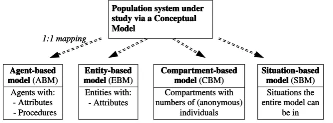
Thus, the choice of representation is mainly about how and where to locate the attributes and procedures of the subjects. There are four possible representations, which we denote: Agent-based, Entity-based, Compart-ment-based and Situation-based. Because the representation has such a profound impact on the model, we also classify the models according to their representation as Agent-based, Entity-based, Compartment-based, and Situation-based models, abbreviated ABM, EBM, CBM and SBM, respectively4. Figure 3 shows these four types of model representations.
Agent-based representation (ABM)
The agent-based representation is the most straightforward. Here an object with its properties and behaviours of interest is represented by a one-to-one mapping to a subject with attributes and procedure(s). The agents may interact with other agents and with their surroundings, and may also be affected by their surroundings [12].
Entity-based representation (EBM)
In an entity-based representation, the subject is an entity with attributes but no internal procedure. In this re-presentation, entities with the same or similar behaviours can share an external procedure or logical track system of connected stations (stages) where the entities can move around. The sojourn time in a stage can have any dis-tribution of non-negative values. In both ABM and EBM, each subject can be monitored and referred to [34].
Compartment-based representation (CBM)
In a compartment-based representation, the subject is an anonymous token without any internal attributes and procedure. Here too, the subject’s procedure is an external track system of interconnected stages (not yet com-partments) where the tokens can reside. The subject’s set of possible attribute values is defined by the present stage in which it is residing. In a compartment-based model, a stage contains the number of subjects residing in it, so the individual token is anonymous and cannot be individually followed over time.
For example, if the subjects” attributes are sex, age group and health status that can take the values {Male,
Female}, {Child, Adult, Old} and {Healthy, Sick}, then 2 × 3 × 2 = 12 stages are required to represent all sets (combinations) of attribute values. If the study object is a woman, 27 years of age and sick, her corresponding subject in the model will be located in the stage “Female & Adult & Sick”. Thus the number of stages increases multiplicatively with the number of (discretised) attributes studied. This is called attribute expansion; see [24].
For a compartment-based representation there is also another a complication: a stage is in general NOT a compartment, because a stage has a specific sojourn time distribution (e.g. Weibull, Erlang or an empirical dis-tribution) and a compartment by nature has an exponential time distribution. Technically, it is necessary to use the exponential sojourn time distribution for a compartment, because this is the only memoryless continuous time distribution [5]. It is the memorylessness that allows superposition, whereby newcomers can mix with those already residing in the compartment without distorting the remaining time to departure. The solution to this
[image:12.595.150.483.566.689.2]
67
dilemma is to represent the stage by a structure of compartments in series and/or parallel to approximate the in-tended sojourn time distribution of the stage. This is denoted stage to compartment expansion (or distribution expansion), see [24].
To simulate a compartment-based model, the model must be translated into difference equations (where the state variables are the compartments) to calculate the development over time [35].
Situation-based representation (SBM)
In a situation-based representation, each situation that the entire system can take (as defined by the conceptual model) must be described5. Markov chain models [36] and chain-binomial models [37] belong to this type of re-presentation. A situation-based model is closely related to the compartment-based model. Here too, the subjects are anonymous and only implicitly represented as part of a number. Again, it is crucial here to consider the so-journ time distributions of the stages—although these are often erroneously neglected. However, in contrast to a CBM, where the number of compartments is independent of the size of the population under study, the com-plexity and the size of an SBM grows combinationally with the population size.
In a situation-based model, the possible numbers of subjects in all compartments have to be combined to de-scribe all situations the model can be in. For example, in a model with two interconnected compartments (A and B) and one subject, there are two situations to consider: the subject being in A or in B. With two subjects there are three situations: {A = 0 & B = 2, A = 1 & B = 1, A = 2 & B = 0}, but with n subjects to be distributed into k
compartments there are n + k − 1 over k − 1 situations (“states” in Markov model terminology). Thus, the
num-ber of situations grows combinationally with both the numnum-ber of compartments (in a corresponding compart-ment-based model) and with the number of subjects. Therefore, even a rather small compartcompart-ment-based model may require a huge number of situations to be represented in a corresponding situation-based model. We call this expansion in model size combinational expansion, see [24].
There are two methods of solving/executing an SBM: The first method is to mathematically take the Cartesian product of the situation (“state”) row-vector s(t) at time t and a transition matrix T to calculate the new situation vector s(t + 1). The elements in the situation vector then represent the probabilities of being at every possible situation. The transition elements Tij are the conditional probabilities of moving to situation sj(t + 1) when in si(t).
In this way, all information is obtained in one sequence of calculations; t = 0, 1, 2, ... However, the situation vector and the transition matrix become huge even for rather small models if the population is not very small.
The second way is to use simulation to follow the development from situation to situation over time, by using random numbers to decide the next situation. The situation vector s(t) is then binary, with a single “1” at loca-tion i, representing the actual situation and all other elements being equal to zero. The situation row vector the-reby selects the ith row of the transition matrix, T. A random number, drawn from the pdf represented by the ith row of T, decides which transition will be realised to create a new binary situation vector s(t + 1). In this way a “trajectory of situations” s(0), s(1), s(2), ... is created for each replication. This method requires a large number of replications, but is usually considerably faster than updating the whole pdf for a medium-sized SBM. Of course, some thousands of replications will not cover the whole “situation space”—but that is seldom required for achieving the purpose of the study. Situations are usually aggregated into more relevant measures, e.g. the purpose may be to study the number of infectious subjects in a SIR model where post-analysis aggregation is made over e.g. sexes and ages.
Hybrid representations
Other model approaches that are hybrids of those presented above can be used for simulation, for example Petri nets [38]. See Appendix C.
4.2.4. Relations between Model Representations
To illustrate the four types of representation introduced above, how they are related and how they can be trans-formed by straightforward mapping of ABM via EBM and CBM into the most abstract SBM, we present the following example.
Example 1: Relations between model representations
A conceptual SIR model is an epidemic model composed of three stages: S (Susceptible), I (Infectious) and R
(Recovered). In the particular population model considered here, each of 11 subjects meets everybody else. A
5The situation is usually called “state”, a word we try to avoid in this paper because “state” has different meanings indifferent
68
[image:14.595.140.484.395.650.2]Susceptible subject becomes infected by an Infectious subject with a specified probability per time unit and an Infectious subject recovers according to an assumed sojourn time distribution. This type of model was first for-mulated by W.O. Kermack and A.G. McKendrick [39]. To the stage attribute = {S, I, R} here we add the attribute sex = {Male, Female}. Furthermore, we specify the sojourn time of the Infectious stage as having the same 3-Erlang distributions for both males and females. Thus the infectious stage must be represented by three serially connected compartments in CBM [40]. InFigure 4 this conceptual model is represented as ABM, EBM, CBM and SBM.
Figure 4demonstrates a sequence of transitions (T1 to T6) from one representation to another. It shows how an ABM of an infectious population can be stepwise translated via EBM and CBM into an SBM. The figure can be interpreted in the following way:
The ABM is just a 1:1 mapping of the Conceptual model described above. Each subject is represented as an agent with its attributes (Health status: {S, I, R} and Sex: {Male, Female}) and procedure (S →I →R), where the sojourn time distribution in the Infectious stage is considered. The S and R stages have no such defined so-journ time distributions.
T1 (inside out): The ABM can be transformed by T1 so that each agent is turned inside out in the sense that instead of having n agents with internal procedures (S →I →R), the procedures, in the form of n track systems, become external. Now these n procedures contain one subject each, placed in their current stages; S, I or R. The sex attribute, which remains unchanged, is still located within each subject.
T2 (Superposition): Next, the n track systems, one for each subject, are super-positioned into a common track system where each of the n subjects is located at its stage. We thereby obtain an EBM with entities whose sex attribute preserves their values of male or female.
T3 (Attribute expansion): The EBM can then be transformed so that it is expanded according to the attribute values {Male, Female}. Attribute expansion can be “costly” when there are several attributes that can take many values (or intervals of values if the attributes take continuous values). For example, with the attributes K, L and M taking k, l and m different values, respectively, the size of the model structure is multiplied by a factor of
69
k ×l ×m. The attributes of the former entities are now handled by the stages containing tokens without any re-maining attributes. These tokens can still be referenced. (In a general case, when an attribute takes continuous values, e.g. age, then the necessary discretisation into intervals would mean some loss of information.)
T4 (Identity loss): In this transformation, the identities of (references to) the tokens are dropped and replaced by a number of tokens in each stage. For a large number of tokens this can result in a considerable reduction in model size. However, this drop of information making the tokens anonymous also means that it is no longer possible to follow a particular token over time. For example, it is no longer possible to find the token with the longest time in the infectious stage, or even to calculate the length of this time.
T5 (Stage to compartment expansion): The stage to compartment expansion (also called distribution expan-sion) is necessary because the individual tokens are anonymous. When a token enters a stage for a sojourn ac-cording to a specific sojourn time distribution, it is no longer possible to keep track of its sojourn in the stage. Furthermore, to allow mixing of newcomers and tokens that have been in a compartment for some time, it is mathematically necessary that the sojourn times in a compartment have a memoryless, i.e. exponential, sojourn time distribution. Therefore, the infectious stage must be represented by a structure of three serial compartments with the time constants T/3 to produce the intended 3-Erlang(T/3) sojourn time distribution of the infectious stage. The transformations T3, T4 and T5 take the EBM into a CBM. (In a general case, representing a given sojourn time distribution by a structure of compartments implies an approximation.)
T6 (Combinational expansion): Finally, a CBM with k physically interconnected compartments that is po-pulated by n anonymous tokens can be in n + k − 1 over k − 1 discrete situations. In our example, we have two
separate compartment chains for male and female tokens, respectively—although linked since a male can infect a female and vice versa. A graph or a situation vector (“state vector”) representing these situations can be used to represent all possible situations the total model can be in. By connecting these situations to describe possible transitions and by including the probabilities of each transition between pairs of situations, a “state”-transition graph is obtained. It is also possible to use a transition matrix composed of transition probabilities that can up-date the situation (“state”) vector over time. We now have an SBM.
Note, however, that if one starts by observing, measuring or estimating the individual transition probabilities of a transition graph (or matrix), then the assigned transition probabilities will lack the consistent couplings ob-tained if the SBS is derived from a CBM. This almost certainly implies that there will be no CBM that exactly corresponds to the SBM. (However, one can find a CBM that best, in e.g. a least squares sense, corresponds to the SBM.)
Thus, a representation can be obtained from a sequence of transformations. For example: the SBM represen-tation can be derived as T6[T5[T4[T3[T2[T1[ABM representation]]]]]]. These transformations preserve con-sistency of results from ABM, EBM, CBM and SBM, provided that the transformations are properly performed.
In this example, all transitions except T4, where identity was dropped, and T6 are reversible (symbolised by two-way arrows). In fact if the SBM equals T6 [CBM] it is reversible, but an empirically obtained SBM usually has no exactly corresponding CBM. ■ In a general case, an attribute expansion of a continuous attribute will introduce some attribute discretisation error in T3. However, the discretisation error can be reduced by using a finer subdivision of attribute values. Moreover, the stage to compartment expansion T5, where a stage is represented by a structure of compartments to approximate the sojourn time distribution, is only exact for the Erlang type of distribution. Such an error can be made arbitrarily small at the expense of a more complex stage description.
4.2.5. Choice of a Proper Model Representation
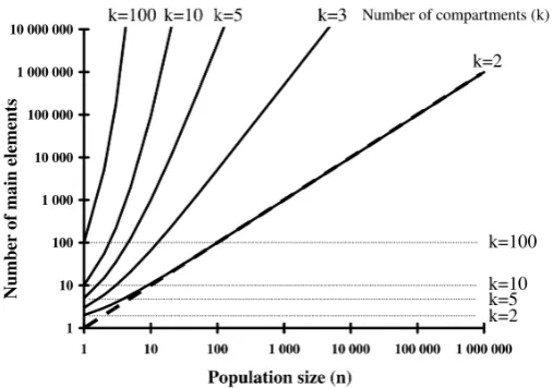
How ABM & EBM, CBM and SBM grow in size for a modelled population of n subjects requiring k compart-ments is shown inFigure 5. The number of situations is in this case based on the assumption that each of the n
subjects can populate any of the k compartments. Although the elements (agents, entities, compartments or situ-ations) are different concepts from different model representations, the figure illustrates the number of main elements required for each representation.
70
Figure 5. The number of components required for agent and entity-based (dashed line), compartment-based (dotted lines) and situation-based (solid lines) models of a population under study, where nsubjects require k interconnected compartments.
The number of situations is based on the assumption that each of the n subjects can populate every of the k compartments.
awkward for simulation modelling, and they also have a number of additional disadvantages related to stochas-ticity and time handling [24].
The choice between ABM, EBM and CBM has its pros and cons. FromFigure 5, we see that the size of an ABM and an EBM both grow linearly with the size of the population under study, while a CBM remains con-stant in size. On the other hand, the number of compartments in a CBM grows multiplicatively with the number of possible values of each attribute, as well as with the complexity of stages (modelled as structures of com-partments). These factors only marginally affect the complexity of agents or entities of an ABM or an EBM. The question of attributes is one of homogeneity; with few attributes to consider, we obtain a rather homogeneous population model, making a CBM an attractive option.
Another issue is whether identity must be preserved in the model. If this is the case, it will exclude the use of a CBM (and of an SBM).
The choice between ABM and EBM is often a matter of taste. However, procedural homogeneity (so that all subjects can use the same track system) makes an EBM attractive. An ABM, on the other hand, is a good choice if there are many types of subjects and if the modeller needs to write his or her own code that is not supported by the multitude of standard stages (stations) and transition mechanisms in an entity-based simulation language.
The type of question to be studied is also important. The use of an ABM or EBM offers the opportunity to add details, heterogeneity and complexity to the behaviour of the individuals and to study the consequences of these additions. However, complexity may also make it difficult to distinguish important patterns.
An ABM and an EBM describe the population on an individual level, while a CBM focuses on subpopula-tions having the same set of attribute values, which may be the level of the system under study we are interested in. In such a case, using an ABM or EBM to generate the subpopulations is a detour. For example, it is argued by Grimm [41] that in ecological models, “bottom-up approaches [individual-based models] alone will never lead to theories at the system level”, and that “state variable or top-down approaches [CBMs] are needed to pro-vide an appropriate integrated view”.
The transformations introduced in Section 4.2.4 are important for translation between representations. They show how a CBM can be constructed consistently with a corresponding ABM, except that the possibility to track individuals is lost.
Furthermore, in Chapter 5 we show how a stochastic CBM can sometimes be approximated by continuous and deterministic flow models that are easier to analyse mathematically. Such an approximation results in loss of information, however.
4.3. Handling Uncertainties
71
available. Describing only the causal relations between different components of the system under study (as we understand it) provides a deterministic model. Compared with the behaviour of the deterministic model, the be-haviour of the system under study will in many cases look somewhat irregular. However, there is information in these irregularities—even when they are too complex to understand and to model in detail—that can be at least partly reproduced by statistical distributions and can therefore be used in the model. Technically, this can be ac-complished by describing the relevant statistical distribution and then using it in the generation of random num-bers. We thereby obtain an irregularly behaving stochastic model of the system under study that will behave somewhat differently for each simulation run (replication).
4.3.1. Handling Different Types of Uncertainty
In our next example, we discuss where uncertainty can appear in discrete population modelling by considering the five types of uncertainty introduced in Chapter 3: Structural uncertainty, Transition uncertainty, Initial value uncertainty, Parameter uncertainty and Signal uncertainty. We then discuss how these types of uncertainty can be handled.
Example 2: Representation of uncertainties
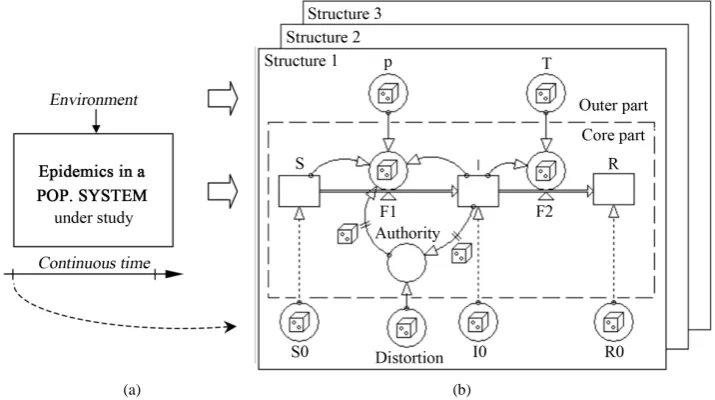
An epidemic in a population system is studied by a model similar to that in Example 1, but with no sex attribute and where the sojourn time distribution in the infectious stage is uncertain. In addition, we include an authority that collects information about the number of infectious individuals and issues recommendations about avoiding contact and using sanitary measures, which affects the infection rate. This is shown inFigure 6. The model is used to demonstrate the locations of the uncertainties and how they can be handled in the model. Here we choose to use a CBM to demonstrate where and how these uncertainties can enter the model, although we could also have used an ABM or EBM.
Structural uncertainty about the system under study can be handled by alternative models. The uncertainty is then reflected by the difference in behaviour of these models.
The remaining four types of uncertainty are handled within the model by assigning probability distributions. By drawing random numbers from these distributions we introduce Transition, Initial value, Parameter and
Signal stochasticities. We now have a stochastic model that behaves differently for each replication.
Technically, a compartment-based model is composed of stages, transitions, parameters and information links. Each of these composition elements can have its own type of uncertainty. Approximate information about the number of objects in the stages at time zero can motivate initial value stochasticities for S(0), I(0) and R(0). There is almost never enough information to decide the exact event times for transitions. Therefore, transition
[image:17.595.135.493.473.673.2](a) (b)
Figure 6.Example 2. (a) An infectious system under study and its environment. (b) Alternative epidemic models, the first of which is a SIR model based on the stages S, I and R (initiated to S0, I0 and R0), transitions F1and F2, and parameters p, T and Distortion. An “Authority”, collects information about the number of infectious individuals and issues recommendations,
72
stochasticity6 in the flows F1 and F2 is used to complement the dynamic description with the available statistical information for the transitions. Unexplained irregularly varying values of the parameters p, T and Distortion
motivate the use of parameter stochasticity6 to generate realistic inputs from these parameters. Uncertainty about the delay of a signal can be described by signal stochasticity. The locations of the stochasticities are sym-bolised by dice inFigure 6(b).
The dashed rectangle in Figure 6(b) approximately represents the system under study inFigure 6(a). This
core part of the model is the explained part, consisting of dynamic relations. This part may contain uncertainties in transitions of subjects or signals because of a high aggregation level.
The outer part of the model contains supplementary unexplained influences on the core part of the model that we have no intention to structurally model. Here we only describe the influences from the environment and the conditions at time zero as parameters and initial values, if necessary in statistical terms. ■
4.3.2. Handling Structural Uncertainty
The description of the SIR model in Example 2 is not complete. In particular, the time in the Infectious stage (the so-called sojourn time) is on average T time units. However, some individuals will recover sooner and oth-ers will require a longer time. By modelling the Infectious stage by a single compartment (as is done in “Struc-ture 1” ofFigure 6(b)), we implicitly assume an exponential sojourn time distribution. Other assumptions about this distribution can be realised by using several compartments in parallel and/or series.
Another structural possibility is that an infected individual does not immediately become infectious. The ex-posed individual may require a latent period before entering the Infectious stage. This can be accomplished by including an Exposed (E) stage between the Susceptible and the Infectious stages (giving a so-called SEIR mod-el).
By studying the differences in outcomes (size of the epidemic, time until the last person recovers etc.) for the alternative models, it is possible to create an estimate about the contribution to uncertainty in the results that comes from structural uncertainty.
4.3.3. Handling Transition Uncertainty
Subjects can instantly change from one stage to another. The change of a subject is an event that takes place at a point in time called the event time. Such events may occur regularly or irregularly in time. The rate (number of events per time unit) of subjects transferred from one stage to another is called the intensity.
Transition uncertainty is handled by transition stochasticity. If we know the expected intensity, which may vary over time, then the number of independently occuring transitions during a short time step is obtained by drawing a “random” number from a Poisson distribution with the intensity as argument. (Equivalently, the in-terval between two successive transition events may be generated by drawing from an exponential distribution with a time parameter equal to the inverted value of the intensity.)
The expected intensity is in turn given by some expression where stochastic parameters (Parameter stochas-ticity) can also be included. SeeFigure 6(b).
A transition event takes a different expression in different representations.
For an agent-based model, a transition event will change the value of the stage attribute of a specific agent.
For an entity-based model, a transition event will change the stage of a specific entity.
In a compartment-based model, anonymous subjects are transferred from one stage to another. When a stage is expanded into a structure of compartments, there will also be internal stochastic transitions between the compartments representing the stage.
In a situation-based model, a situation refers to the entire model, so an event affecting any subject will take the model from one situation to another.
Transition stochasticity is the driving force in a stochastic discrete model. Without the irregularly occurring transition events, no development over time will take place in such a model. Thus, the transition stochasticity generates both the dynamics of the model and the stochastic development in an inseparable way7.
The technical realisation of transition stochasticity depends on the time handling principle used. Because time
6Transition stochasticity is often called demographic stochasticity and parameter stochasticity is often called environmental stochasticity in
biological and ecological population models, see e.g. [6] [42].
7This inseparability is important. There are many awkward examples of trying to separate dynamics and stochastics by adding stochastic


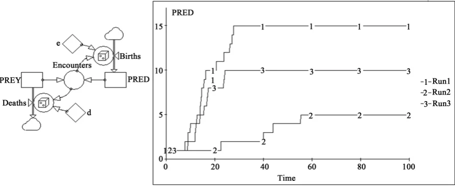
![Figure 9. A Forrester diagram [51] of a stochastic logistic model and the results of three replications of the model for the case a = 0.1, b = 0.01 and x(0) = 1](https://thumb-us.123doks.com/thumbv2/123dok_us/7954925.752533/26.595.91.538.481.694/figure-forrester-diagram-stochastic-logistic-model-results-replications.webp)