A closed form solution to Stollery's global warming problem with temperature in utility

Munich Personal RePEc Archive

A closed form solution to Stollery’s

global warming problem with

temperature in utility

Bazhanov, Andrei

Far Eastern National University, Queen’s University, Kingston,

Canada

29 April 2010

Online at

https://mpra.ub.uni-muenchen.de/22406/

A closed form solution to Stollery’s global warming

problem with temperature in utility

Andrei V. Bazhanov

a_{Far Eastern National University, Vladivostok, Russia}

b_{Department of Mathematics and Statistics, Queen’s University, Kingston, ON, K7L 3N6,}

Canada

Abstract

Stollery (1998) studied a polluting oil extracting economy governed by the

con-stant utility criterion. The pollution caused the growth of temperature,

nega-tively a¤ecting production and utility. Stollery provided a closed form solution

for the case with the Cobb-Douglas production function and temperature

a¤ect-ing only production. This paper o¤ers a closed form solution to a non-trivial

example of this economy with utility a¤ected by temperature.

Key words: essential nonrenewable resource; polluting economy; sustainable

development; special function representation

1. Introduction

A social planner in Stollery’s (1998) problem followed a constant utility

criterion where utility and production were negatively a¤ected by irreversible

global warming resulting from oil use. Stollery obtained the closed form

so-lutions, considering the case with temperature a¤ecting only production for

the extended Dasgupta-Heal-Solow-Stiglitz (DHSS) model (Dasgupta and Heal,

1974; Solow, 1974; Stiglitz, 1974) under the Hartwick investment rule (Hartwick,

1977).1 _{Stollery did not consider the case where temperature a¤ected utility,}

noting that “exactly the same energy path results from temperature e¤ects in

a standard constant elasticity utility function” (Stollery, 1998, p. 734).

However, the case with utility a¤ected by global warming raises some

in-teresting and important questions since the negative e¤ect of temperature can

represent an aggregate damage resulting from economic activity. For example,

Bazhanov (2009b) analyzed a solution to this problem for an imperfect

econ-omy that has been extracting the resource for a period of time before considering

the goal of sustainable development in the form of the constant utility criterion.

This approach showed that the economy can be sustainable or unsustainable

de-pending on the parameters of the hazard function and on the technology and the

initial endowments of the economy. The result implied the necessity of a more

general notion of sustainability (semisustainability) that can provide an

oppor-tunity for an economy to decline asymptotically to a su¢cient survival level

instead of collapsing in …nite time after a period of overconsumption. A similar

problem arises in the cases when utility is positively a¤ected by the remaining

resource stock, e.g., when the stock has an amenity value (Krautkraemer, 1985;

Schubert and d’Autume, 2008).

In Bazhanov (2009b), the problem was studied numerically using a

di¤eren-tial equation for capital, which implied all other paths in the economy including

the path of the hazard function. The current paper provides the closed form

solution for a speci…c case in this economy. Unlike Bazhanov (2009b), where

the problem was formulated for an imperfect economy with the given state of

the oil extraction industry (the initial rate of extraction), this paper o¤ers a

conventionally speci…ed example for the given initial assets of capital and the

resource reserve. The uncertainty of policy recommendations in this case is

discussed using a numerical example, which resembles the current state of the

world’s oil extracting industry.

2. The model

Stollery provided a closed form solution to an oil-burning DHSS economy2

with the production function negatively a¤ected by growing temperature and

with an isoelastic utility that depended only on consumption. The current paper

considers the case with utility alone a¤ected by the hazard functionT:A social

planner chooses the path of per capita consumption c (by choosing a saving

rule) and the path of the per capita resource extractionr (by choosing a tax)

to maximize the constant over time level of per capita utilityu:

u(c; T) = cT 1 (1 )=(1 ) =u=const[c(t); r(t)]! max

c(t);r(t): (1)

The balance equation and the production function are

q(t) =c(t) + _k(t) =k (t)r (t); (2)

whereqandkare per capita output and capital; ; 2(0;1); + <1; > :3

The optimal investment rule is k_ := dk=dt = rqr = q; where qr := @q=@r:

Stollery assumed that technical change compensated for the e¤ect of growing

2_{The Cobb-Douglas production function, which is used in the DHSS model, has become one}

of the most popular tools in Resource Economics both for theoretical studies (e.g., Dasgupta and Heal, 1979; Asheim, 2005, Hamilton and Withagen, 2007) and for practical applications, e.g., for the global climate change assessment (Nordhaus and Boyer, 2000).

3_{The share of labor in this problem is 1 :The Solow (1974) condition >}

population, so there are no explicit technical advances in the model, and

popu-lation is constant.4 _{The hazardT grows with the resource extraction:}

T(t) =T[r(t)] =T0

Z t

0

r( )d + 1

'

=T0[ (s0 s(t)) + 1]'_{; (3)}

where ; ' > 0 are the parameters, s0 is the initial per capita oil stock, and

s= s(t) is the current oil stock, implyingr = s:_ Function T can vary from

constant to polynomial depending on the value of':5

The constant utility criterion requires the following paths of per capita

out-putq;consumptionc;and, di¤erentiatingq;the path of the growth rateq=q_ :

q(t) = q0f [s0 s(t)] + 1g'; (4)

c(t) = c0f [s0 s(t)] + 1g'; (5)

_

q(t)

q(t) =

' r(t)

[s0 s(t)] + 1: (6)

The rate of growth for' >0is positive, declining starting from

_

q(0)

q(0) =' r0; (7)

and approaching zero with t ! 1: The optimal initial consumption is c0 = (1 )q0; where q0 = k0r0; and the value of the initial rate of extraction

r0=r0(k0; s0; '; )is linked to the initial stocks and the intensity of the hazard

via the e¢ciency conditions0=R₀1r(t)dt:6

In contrast to the Solow-Hartwick case (' = 0), per capita output and

consumption grow here under the same Hartwick investment rule when' >0:

The growth is limited by

q1 = q0f s0+ 1g

'

and (8)

c1 = c0f s0+ 1g

'

(9)

4_{A plausible alternative to this assumption can be a TFP (Total Factor Productivity)}

compensating for capital decay. In more details see Bazhanov (2009a).

5_{The speci…cations of utility and temperature functions are di¤erent here from the ones}

considered by Stollery; in particular, Stollery related temperature to the remaining resource stock (T0

(s(t)) < 0); here temperature depends on the extracted (burned) resource stock (T0

(s0 s(t))>0). The other di¤erences are discussed in Bazhanov (2009b).

respectively. The limit for temperature growth is T1 = T0(s0 + 1)

'

: The

only source of output and consumption growth is a redistribution of the

re-source among generations. A social planner imposes a positive declining tax on

extraction, resulting in a lower rate of initial extraction (implying lowerc0and

q0) and a slower decline in the rates of extraction. Namely, from the speci…-cation of the production function, the equation for the rate of output growth

isq=q_ = k=k_ + r=r:_ Then, given k0_ = q0 and using (7), the initial rate of

change in the rate of extraction isr0=r0_ = [' r0 q0=k0]= or

_

r0 r0 =

r0h

' k0 1r 1 0

i

yielding the following condition:

_

r0R0 i¤ ' R

k01 r 1 0

: (10)

This condition, however, does not directly imply that a growing initial extraction

can be optimal in this problem becauser0 declines with the growth of ' :A

speci…c example of the optimalr0_ >0is provided in Section 4, condition (42).

The growth of output and the declining to zero ‡ow of the resource imply

an unbounded growth of capital in this problem.

The constant-utility criterion in the form of (1) seemingly implies that the

optimal initial values of q0 =c0=(1 ) and c0 should depend on the

prefer-ence parameter and the initial temperatureT0;namely,cT 1_=ub=const=

[u(1 )]1=(1 ) yielding c0 =T0[u(1 )]1=(1 ): However, since is a con-stant here, the optimal policy in this framework maximizes u_b and the

corre-sponding value of u(u;b ) regardless of the preference parameter. As to the

value ofT0 as a “preindustrial level” of temperature, the normalizationT0= 1

can be used assuming that the hazard does not a¤ect utility when the resource is

not being extracted. Hence, problem (1) is equivalent to the problem of …nding

b

u=const[c(t); r(t)] = max

c(t);r(t)c(t)T[r(t)] 1

(11)

For obtaining the optimality conditions, Stollery used the approach of Leonard

and Long (1992, pp. 300-304), which reformulates problem (11) into the

follow-ing equivalent problem:

maximize V(t)

Z 1

t b

u e d fort= 0 (V(0) =bu=const) (12)

for an arbitrary constant subject to (omitting the dependence on time)

_

k=q c; s_= r; andub=u(c; T): (13)

The Hamiltonian of this problem is

H =u eb t+ k(q c) sr: (14)

The utility constraint yields the Lagrangian to be maximized:

L=H+ (u bu):

In the general case, when both production and utility are a¤ected by the hazard,

the Pontryagin-type necessary conditions for the state variablesk andsare7

Lc= uc k = 0; (15)

Lr= kqr s= 0; (16)

_k =

@L

@k = kqk; (17)

_s=

@L

@s = ( kqT+ uT)Ts0 s @(s0 s)=@s; (18)

Z 1

0

Lbudt=

Z 1

0

e t dt= 1

Z 1

0

dt= 0: (19)

Eq. (18) with k from Eq. (15) results in

_s=Ts0 s uc qT +

uT

uc

: (20)

7_Here

k and s are indexed dual variables unlike uc; qk;andqr;which are the partial

The time derivative of Eq. (16) is _s= _kqr+ kq_r;which, divided by qr and

combined with Eq. (20), gives

_

qr

qr k

+ _k =

Ts0 s uc

qr

qT +

uT

uc

:

Substitution for _k from Eq. (17) with k from Eq. (15) yields

_

qr

qr

=qk+

Ts0 s

qr

qT +

uT

uc

; (21)

which is the Hotelling rule with the negative additional term (t) :=Ts0 s(qT +uT=uc)=qr

resulting from the e¤ects of the externality. The fact that (t)6= 0in the pres-ence of the hazard factor (' > 0) implies that the optimal paths in this

problem can only be asymptotically e¢cient because the standard Hotelling

rule ( = 0) as a necessary e¢ciency condition8 _{is satis…ed only with t ! 1}

due to exhaustion of the resource.

Stollery obtained the optimality of the Hartwick rule from the

Hamilton-Jacobi-Bellman equation9 _{for the problem (12), (13) instead of using necessary}

conditions (15) – (19). Namely, the Hamilton-Jacobi-Bellman equation

estab-lishes the following link between the maximized Hamiltonian and value function:

@V =@t=H : (22)

An autonomous in…nite-horizon problem such as (12), (13) has the property:

V(t) =V(0)e t_:10 _{Then @V =@t=V(0) e} t_{=bu e} t_{and H =bu e} t₊

Vkk_+Vss_ ( k and s are the shadow prices of capital and the resource stock)

yielding _kk_+ ss_= 0, which means that the investment kk_ must be equal to

the resource rent srunder optimal prices (Hartwick, 1977).

In this framework, the equations for the optimal paths in the economy can

be derived from

a) the conditioncT 1_=bu=const;

b) the Hartwick rule, which provides the maximum level ofu;b

8_{See, e.g., Dasgupta and Heal (1979).}

c) the balance equation (2) specifying the production function, and

d) the Hotelling rule (21), which gives the optimal tax on extraction.

3. Optimal paths

The optimal path of output (4) can be written asq(t) =q0h R₀tr( )d + 1i

'

:

Raising to the power1='yieldsq1='_=q1='

0

h Rt

0r( )d + 1

i

(restriction'6= 0

will be lifted below). Time derivative, substituting for r = q1= _k = _{; is}

q1=' 1_{q='_ =q}1=' 0 r=q

1='

0 q1= k = :This equation with the optimal saving

rule gives a system of the two di¤erential equations inqandk:

q1=' 1 1= dq=dt = 'q10=' k = ;

dk=dt = q:

Following Schubert and d’Autume (2008), the system can be solved by

elimi-nating time (dt=dk=( q)): q1=' 1= _dq=A1k = _{dk;whereA1='q}1='

0 = >

0: Integration gives q1+1=' 1= _{=(1 + 1=' 1= ) = A1k}1 = _{=(1 = ) +C1}

or qa _=A2k1 = _{+C2;where a= 1 + 1=' 1= = ['( 1) + ]=(' )and}

A2 = aA1=(1 = ): Note that a R 0 and A2 Q 0 when ' Q =(1 ):

Calibration at t = 0 gives C2 = qa

0(1 B1k 1 =

0 ); where B1 = A2q

a

0 = q₀1= 1 ['(1= 1) 1]=( )(B1R0 whenA2R0). Then

q=q0 B1k ( = 1)+C3 b; (23)

where C3 = 1 B1k1₀ = and b = 1=a =' =['( 1) + ]: Henceforth, the

restriction'6= 0 is not relevant; the case with'! =(1 ) causingb! 1

is considered below.

Eq. (23) shows that q(t) ! q = q0Cb

3; and the saving rule implies that c(t)!c =q0(1 )Cb

3 ask(t)! 1witht! 1:The obtained expression for qcombined with the optimal saving rule gives a di¤erential equation in capital,

and then the dynamics of the economy is de…ned by the following system:

_

k = k0_ B1k ( = 1)+C3

b

; (24)

wherek0_ = _k(0) = q0:

The case with'= 0impliesb= 0;yielding linear capitalk(t) = q0t+k0;

which coincides with the Solow-Hartwick case and with Stollery’s solution for

= 0:The extraction in this case isr(t) =r0(r1t+ 1) = ;wherer1= q0=k0:

For the case with'! =(1 );implyinga!0orb! 1;Eq. (24) can be rewritten as follows: k_ = _k0Cb

3 1 +k ( = 1)B1=C3

b

ork_ = _k0Cb

3 1 k ( = 1)aB5 1=a

;

where B5 := q₀aA1=h( 1)C3i: Note that C3 ! 1 when a !0; but Cb

3 =

(1 +aB6k₀( = 1))1=a_{; where B6 := q} a

0 A1=( 1) > 0; so lima!0 C3b =

exphB6k0( = 1)

i

andlima!0B5=B6:Then, Eq. (24) takes the form

_

k= _k0eB6k0( = 1)e B6k ( = 1)_{: (26)}

Eq. (24) is integrable in quadratures:

Z k(t)

k0

d{

B1{ ( = 1)+C3

b = _k0t+Const; (27)

however, in the general case, k(t) obtained from this equation cannot be

ex-pressed in elementary functions.11 _{The following section provides a nontrivial}

('6= 0) example with the closed form solution to Eq. (24).

A di¤erential equation for the tax on extraction (t)can be obtained from

Eq. (21) using the fact that the resource price with no imperfectionsqr

should satisfy the standard Hotelling rule ( 0):

d(qr )=dt

qr

=qk:

1 1_{The LHS of Eq. (27) can be expressed using special functions. For}

ex-ample, in the case with a = 0; this equation takes the form of a nonlin-ear equation in k : z(k) = k_0exp(B6k0( = 1))t + Const; where z(k) =

D1(k) B6k =(1 + ) + 1 W hittakerM(D2; D3; B6k ) + (1 + ) W hittakerM D2+ 1; D3; B6k ;

with := 1 = ; D1(k) := B6(1+3 )=(2 )k(1 3 )=2exp B6k =2 =(1 + 2 );

D2 := (2 )=(2 ); D3 := (1 + 2 )=(2 ): Here W hittakerM( ) is the Whittaker M

special function, which is available, e.g., in Maple or Mathematica software. Whena= 0

and = 2 ;the LHS of Eq. (27) isz_{(k) =kexp( B6=k) Ei(1; B6=k);whereEi( )is the}

This equation gives the dynamic condition for the tax depending on the path

of the Hotelling rule modi…er (t) :

_ _{qk qr= 0: (28)}

Eq. (28) has a solution12

(t) = 0(k(t)=k0) = qr(t) h

(q(t)=q0)1= 1 1i; (29)

where 0= (0)is the initial condition.

The value of 0 can be expressed from the formula for the initial resource

price with no imperfections: qr(0) (0) = q00=r00; where q00 =k0 r00 and

r0

0 satis…es Eq. (32). Namely,

0=

n

k0r 1

0 k0=[s0( )]

o

: (30)

In the case with = 0;there is no tax sincer0=r0

0:Eq. (30) yields the optimal

initial tax that is required to obtain the optimal initial rate of extraction r0;

de…ned in the conventional approach from the e¢ciency condition givenk0; s0; ';

and . Eq. (30) can be inverted to show the link between the value of 0 and

the resulting value ofr0:r0 1= [ 0s0( ) + k0]=[ k0s0( )]or

r0= ( )s0=k

1 0

1 + ( )s0 0=( k0)

1 1

; (31)

which coincides with ther0

0 in the Solow-Hartwick case ( 0= 0)

r00= ( )s0=k01

1

1 ₍₃₂₎

and monotonically declines to zero with 0! 1:

4. An example of a closed form solution

Let '= and = 2 : Then b =a = 1; A2 = aA1=(1 = ) = A1 =

q10= <0; B1=A2q0a = q 1= 1

0 <0; andC3= 1 + k01 r 1

0 >0: In

this case, Eq. (24) becomes

_

k= B4

k +C4; (33)

whereB4 := _k0B1<0 andC4:= _k0C3 >0: Eq. (33) in quadratures, denoting

D0:=B4=C4=B1=C3<0;is

Z

k

k+D0dk=C4t+C;b

whereCb is the constant of integration. Integration of the LHS yields

k D0ln (k+D0) =C4t+C:b (34)

After denoting x:= ln (k+D0); the last equation becomes ex _{D0(x+ 1) =}

C4t+Cb or ex_{=D0(x p);where p:= C4t=D0 1 C=D0:b Multiplication}

of both sides by e x+p_{=D0 results in the equation e}p_{=D0 =e}(p x)_{(p x);}

which, by the de…nition of the Lambert W function,13 _{has the solution}

p x=W( ep=D0):

Then,k+D0 = exp [p W( ep_{=D0)] = D0[ e}p_=D0]e W( ep=D0)_{: The}

def-inition of the Lambert W function implies thatW(z) =ze W(z); transforming the last equation as follows: k+D0= D0W( ep_=D0)or

k(t) = D0

8 <

:1 +W

0

@ e

C4 D0t 1

b C D0

D0

1 A

9 =

;; (35)

where C;b de…ned from Eq. (34) at t = 0; is Cb = k0 D0ln (k0+D0): After

substitution forCbinto Eq. (35), it becomes

k(t) =D0 1 W e DC40t e k0

D0 1 k0

D0 1 ; (36)

which must be equal to k0 at t = 0: Indeed, by the de…nition, W[ez_{z] = z;}

therefore, the RHS of Eq. (36) at t = 0 equals D0n 1 h k0 D0 1

io = k0:

Since C4=D0 < 0; D0 < 0; and W is monotonically growing function with

1 3_{Lambert W function is the solution to the equationye}y _{= z;namely, y =W(z):The}

derivative (forz6= 1=e) ofW is dW=dz=W(z)=[z(1 +W(z))];and the antiderivative of

limz!1W(z) = 1; capital is growing with no limit along a path that grows

faster than a linear function (Fig. 6). Formula (36) can be considered as a

closed form solution fork(t)(using an alternative de…nition of this notion) since

functionW is uniquely de…ned fork0>0;14 _{and numerical implementations of}

this function are available in major computational software.

Substitution fork(t)into Eq. (24) gives the closed form path of investments,

which, using the optimal saving rulek_ = q; implies the paths of output,

con-sumption, and extraction:

q(t) = q0

(

B1

D0 1 W e

C₄ D0t e

k₀

D0 1 k0

D0 1 1

+C3

)

;(37)

c(t) = c0

(

B1

D0 1 W e

C4 D₀t _e

k0

D₀ 1 k0

D0 1 1

+C3

)

;(38)

r(t) = q(t)1= _k(t) = _{; (39)}

wherec0 = (1 )q0:On the other hand, the constant utility criterion implies

thatc(t) =c0[ (s0 s(t)) + 1]'_{;yielding (for'= ) the equation for the path}

of the current reserve:

s(t) =s0 1 nB1k(t) 1+C3o1= 1 :

In the limit, this formula becomes s1 = limt!1s(t) =s0 1 C

1=

3 1 = s0 1 + k10 r

1 0

1=

1 = :Then, the e¢ciency conditions0=R₀1rdt

results in the following relationship betweenk0; s0; andr0:

r0=nh(s0 + 1) 1i= k10

o1=(1 )

: (40)

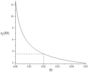
Note thatr0is a decreasing function of in this case (Fig. 1), which means

that the greater the intensity of the hazard the larger the amount of the resource

1 4_{Function W(z) is uniquely de…ned for z > 1=e implying that k}

0 should

sat-isfy the condition e

C4 D0t _e

k0

D0 1 k0

D0 1 > 1=e for any t > 0: This

in-equality holds when k0

D0 1 > 0 or k0 > D0 ( D0 is a positive number here:

D0 = B1=C3 =k0= r

1 0 =

h

1 + k₀1 r1₀ i). Then, after dividing both sides by

k0= 1 + k10 r

1

0 ;the condition of the uniqueness of the representation via the Lambert

that should be left for the future in order to o¤set the hazard with the growth

of consumption according to the criterion. At the same time, reallocation of the

resource to the future ‡attens the path of temperature until the rates of growth

of temperature and consumption completely compensate for each other.

The initial tax on extraction should be higher (Fig. 2) for a larger ; and the initial level of consumption should be lower as a result of a lowerr0. Letting

!0and using the L’Hôpital’s rule, condition (40) becomes

r00= lim_!

0r0= s0=k 1 0

1

1 ₍₄₁₎

coinciding with the expression (32) in the Solow-Hartwick case for = 2 :

Formula (40) speci…es condition (10) of the optimality of the growing

ini-tial extraction depending on the hazard factors. Namely, the second

inequal-ity of this condition becomes R k10 =

n

k10

h

(s0 + 1) 1io or 1 R

=h(s0 + 1) 1i;yielding

_

r0R0 i¤ R (1 + )1= 1

s0 : (42)

According to this condition, the optimal pattern of extraction can be

hump-shaped even in the case with a small intensity of the hazard when the initial

reserves0is large. An example of the optimal hump-shaped extraction path is

provided in the next section (Fig. 4, solid line).

Formula (30) for = 2 becomes

0= k0r 1

0 k0=s0: (43)

The explicit dependence of the initial tax on the hazard parameter results

from combining Eqs. (40) and (43):

0( ) =

k0

(s0 + 1) 1

k0

s0: (44)

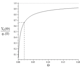
Expressed in the terms of the resource price, the initial tax is 0( )=qr(0) =

1 k01 = s0 r0( ) 1 or

0( )=qr(0) = 1

(s0 + 1) 1

This equation shows (using the L’Hôpital’s rule) that 0( )=qr(0)

asymptoti-cally approaches unity with ! 1starting from zero when = 0(Fig. 2). It can be easily shown that the asymptotes15 _{forq(t)andc(t)given by Eqs.}

(37) and (38) coincide withq1andc1given by formulas (8) and (9) for'= .

For example, q1 =q0C3 =q0 1 + k₀1 r₀1 ; which after substitution for

r0 from formula (40) yields formula (8) with'= :

Given Eq. (29) and the other paths (36) – (39), the path of the tax in terms

of the resource price =qris =qr= 0k = = k0= k r 1 (q=q0)1= 1+1;

which can be rewritten as follows:

(t)

qr(t)

=q(t)1= 1 "

0 k0=

1

q01= 1

#

+ 1: (45)

The boundedness of output in this problem implies the value of the asymptote

for =qr;using Eqs. (8) and (43):

1

qr1

= q11= 1

"

0 k0=

1

q10= 1

# + 1

= 0q

1= 1

0 (s0 + 1) 1

k₀= (s0 + 1) 1 + 1 = r 1 0 q 1=

0 (s0 + 1) 1

q01= 1(s0 + 1) 1

k0=s0 k0=

(s0 + 1)1 + 1

= 1 k

1 =

0 s0 q

1= 1

0 (s0 + 1) 1

= 1 k

1 0

s0 r 1

0 (s0 + 1) 1

;

which after substitution forr0 from Eq. (40) becomes

1

qr1

= 1 1

s0

h

(s0 + 1) (s0 + 1)1 i: (46)

Using the properties of the Lambert W function, it can be shown that for

any parameters of the problem the tax becomes negative in the long run when

>0:Namely, from Eq. (46), the condition that 1=qr1<0 fors0 >0 is

(s0 + 1) (s0 + 1)1 > s0 : The substitutionsp:=s0 + 1and v:=

1 + 1=(p 1) (or =v+ 1 + 1=(p 1)) transform this condition into the

1 5_{The asymptotes follows from the fact thatlim}

Figure 1: The dependence of the initial rate of extractionr0 on the hazard factor :

following form:16 _p v_p 1=(p 1)_{< v(p 1);which can be rewritten as}

vpv_< p 1=(p 1)

p 1 or e

vlnp_{vlnp <} p 1=(p 1)

p 1 lnp:

The de…nition of the Lambert W function yields

vlnp < W( p

1=(p 1)

p 1 lnp) or v <

W( p 1=(p_{p 1}1)lnp)

lnp :

The last inequality in the original variables is

<1 + W h

(s0 +1) 1=s0

s0 ln (s0 + 1) i

ln (s0 + 1) +

1

s0 : (47)

SinceW(zez_{) =z(denotingz:=} 1

s0 ln (s0 + 1)), the numerator of the …rst

fraction in (47) is

W 1

s0 ln (s0 + 1) (s0 + 1)

1=s0 ₌ 1

s0 ln (s0 + 1);

and then condition (47) becomes < 1;which is always true in this problem.

Hence, if >0;there existst >0 such that (t)<0 for anyt>tand for any

values of the parameters in this problem (see, e.g., Fig. 3).

1 6_{The same inequality can be obtained from Eq. (45) as a condition of the existence of the}

Figure 2: The dependence of the initial tax in terms of the initial resource price 0( )=qr(0)

on the hazard factor :

5. Numerical example

Let the shares of capital and the resource are = 0:3 17 _{and = 0:15;the}

hazard function parameters: '= ; = 0:02; T0 = 1;the initial stocks of the

economy: s0 = 371bln t,k0= 14:35:18 _{Formula (40) yields the optimal initial}

rate of extractionr0 = 3:524 bln t/year (cf. r0 = 12:61 bln t/year for = 0;

Fig. 1). This reduced initial extraction results from the tax 0= 0:0756(or in

the terms of the resource price 0=qr(0) = 0:66) applied att= 0and estimated by formula (44).

The externality causes the following deviation from the standard Hotelling

rule att= 0 : (0) =Ts0 s(0)uT(0)=(uc(0)qr(0)) =T0' ( c0=T

2

0)= k0r 1 0 =T0 =

(1 )k0r0 = k0r 1

0 = (1 ) r0 or (0) = 0:0599: Eq. (28) yields

1 7_{See, e.g., Nordhaus and Boyer (2000).}

1 8_{To make the example more illustrative, these initial values imply the rate of extractionr}

0

that is close to the current world oil rate of extraction givens0as the world oil reserve estimate.

Namely, the world rate of crude oil extraction on January 1, 2010 is 70502.6 [1000 b/day]/7.3 [b/t] 365 10 6 _{= 3.525 [bln t/year] (World Oil, 2009). CERA (2006) claimed that}

actual world oil reserve in 2006 was three times larger (about 512 bln t) than the conventional estimate. I take heres0 = 2 185:5 = 371[bln t] = 2 1,354,182,395 [1000 b]/7.3 [b/t]

10 6_{;where 185.5 [bln t] is the conventional estimate (World Oil, 2009). One ton of crude oil}

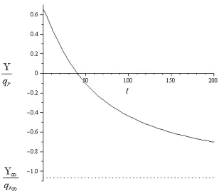
Figure 3: The path of the tax in terms of the resource price (t)=qr(t):In the Solow-Hartwick case the tax is zero.

_ (0) = 0qk(0)+ (0)qr(0):The initial values of marginal productivitiesqk(0) =

k0 1r0 = 0:056 andqr(0) = k0r 1

0 = 0:11 result in _ (0) = 0:0026

show-ing that the tax is declinshow-ing att= 0:

The path of the tax in terms of the resource price (45) is depicted in Fig. 3.

The tax becomes negative after 40 years and approaches the negative asymptote

1=qr1= 1:07:

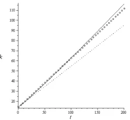
Capital for = 0:02(Fig. 6, solid line) grows faster than a linear function.19

Linear capital in the Solow-Hartwick case (Fig. 6, circles) has a steeper slope

(k_0

0 = 0:488) due to the higher rate of extraction att= 0:The optimal paths of

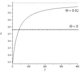
per capita consumption for the cases with = 0:02and = 0are in Fig. 7.

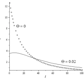
The tax imposed by the planner for = 0:02 results in a hump-shaped

optimal path of extraction (Fig. 4, solid line). The path in circles in Fig. 4

corresponds to the case with = 0(Solow-Hartwick case, no tax). Note that,

in the conventional approach,20 _{a relatively small uncertainty in the hazard}

parameter leads to a large uncertainty in the short-run resource policy (Figs.

2 – 5). The model shows that if the planner is unaware of the externality

1 9_{This linear functionk}

0+ _k0twithk0andk_0= 0:403for = 0:02is depicted as a dotted

line in Fig. 6

2 0_{I mean here the approach wherer}

Figure 4: The optimal paths of extraction: for = 0:02- solid line, for = 0(Solow-Hartwick case) - circles.

or is going to neglect its e¤ect and implement an economic program with the

maximum constant per capita consumption over time, she should apply the

policies that will result in the current rate of extractionr0= 12:61bln t/year, which is 3.6 higher than in the case with = 0:02:

The uncertainty of the conventional approach in de…ning r0 with respect

to the imprecision of the reserve estimate s0 is illustrated in Figs. 5a and 5b,

where s1

0 is a conventional world oil reserve estimate (World Oil, 2009), s30 is

the estimate of CERA (2006), and s2

0 = 2 s10 is the estimate that is used

in this example ass0 and is somewhere betweens1

0 and s30: Note that a small

hazard factor (Fig. 5b) results in higher uncertainty than the large one since,

for the larger values of ; the initial rate of extraction should be essentially

lower, reducing the uncertainty of this value.

For a small extracting …rm that has just discovered or obtained an oil …eld

at an auction, an approach that provides the initial rate of extraction as a policy

recommendation could be possible when the oil-extracting capital is available

in required quantities and the elasticity of the demand for the resource is high.

However, for a large incumbent …rm that has been extracting the resource for

a period of time and is going to reestimate the optimal path, this approach can

Figure 5: The dependence of the initial rate of extractionr0 [bln t/year] on the reserve s0

for di¤erent values of the hazard factors :(a) = 0:02;(b) = 0; s1

0= 185:5bln t – the

current world oil reserve according to World Oil (2009);s2

0= 2 185:5bln t;s30= 512:3bln

t – CERA (2006) world oil reserve estimate.

to uncertainties.

For example, if the extraction was started under the constant consumption

criterion ( = 0) and with the initial reserve estimate s0=s1

0; the initial rate

of extraction would be r1

0 = 5:58 bln t/year (Fig. 5b). The announcement

similar to CERA (2006) about the larger actual reserve s0 = s3

0 would cause

the immediate jump in the rate of extraction up to the new value r3

0 = 18:44

bln t/year as a result of the reestimation of the optimal path using the same

approach. Then, if the social planner takes into account information about the

hazards of the extraction of the resource and decides to follow the constant

utility path with = 0:02;the imposed tax should instantly cut down the rate of extraction to the new initial value_br3

0= 4:2bln t/year (Fig. 5a).

The e¤ect of deviation of the optimal path from the initially estimated path

recalculated at a later date is called “dynamic inconsistency” in the literature.21

In this case, inconsistency takes the form of considerable discontinuous jumps in

2 1_{For example, Newbery (1981) considered various reasons for dynamic inconsistency in oil}

Figure 6: The optimal paths of capital: for = 0:02- solid line, the linear path for = 0

(Solow-Hartwick case) - circles, the pathk0+ _k0twithk0 andk_0 for = 0:02- dotted line.

resource policies that can lead to socioeconomic and environmental damage;22

some of these jumps can be unrealizable in practice.

Hence, the approaches that result in the paths that are discontinuous with

respect to the initial state of economy could be appropriate only for small …rms

entering the market or for theoretical studies where the questions of the

tran-sition to an optimal state are not important (Bazhanov, 2010). In many cases,

reestimation of the optimal path requires a solution that is linked to the

ini-tial conditions, including the iniini-tial state of the extracting industry (Bazhanov,

2009a, Section 9; Bazhanov, 2009b).23

6. Concluding remarks

This paper has o¤ered an example of the closed form solution for the problem

of irreversible global warming under the constant utility criterion (Stollery, 1998)

with utility negatively a¤ected by the hazard factor. The solution was expressed

via the Lambert W special function, which has convenient analytical properties

2 2_{One can recall the consequences of the oil embargo in 1973.}

2 3_{Pezzey (2004, formula (15), p. 477) o¤ered an example of solving the problem of}

Figure 7: The optimal paths of per capita consumption: for = 0:02- solid line with the asymptote (dotted line), the constant path for = 0(Solow-Hartwick case) - circles.

for any parameters in this problem. For example, using the properties of this

function, it was shown that the declining tax in this problem becomes negative

in the long run.

The main qualitative distinctions of this problem from the Solow-Hartwick

case with no hazard are:

(a) output and consumption are growing and asymptotically approaching

positive constants;

(b) the initial rate of the resource extraction is lower, implying (for the same

initial capital) lower levels of initial output and consumption;

(c) the economy is e¢cient only asymptotically with exhaustion of the

pol-luting resource;

(d) the optimal path of the resource extraction can be hump-shaped;

(e) capital is growing faster than a linear function.

The example has shown that the initial rate of extraction and the initial

tax, provided in the conventional approach as policy recommendations, can be

signi…cantly uncertain due to the uncertainties in the initial reserve and in the

intensity of the hazard. The uncertainty is considerably higher in the case of

References

[1] Asheim G. B. 2005. Intergenerational ethics under resource constraints.

Swiss Journal of Economics and Statistics. 141(3), 313–330.

[2] Bazhanov A.V. 2009a. Maximin-optimal sustainable growth in a

resource-based imperfect economy. MPRA Paper No. 19258.

[3] Bazhanov A.V. 2009b. A constant-utility criterion linked to an imperfect

economy a¤ected by irreversible global warming. EERI Research Paper

Series No 03/2009

[4] Bazhanov A.V. 2010. Sustainable growth: Compatibility between a

plausi-ble growth criterion and the initial state. Resources Policy 35(2), in press,

doi:10.1016/j.resourpol.2010.01.002

[5] CERA 2006. Peak oil theory – “world running out of oil soon” – is

faulty; could distort policy & energy debate. Cambridge Energy Research

Associates, Inc. (November 14, 2006). Accessed on March 17, 2010 at

<http://www.cera.com/aspx/cda/public1/news/pressReleases/pressReleaseDetails.aspx?CID=8444>

[6] Corless R. M., Gonnet G. H., Hare D. E. G., Je¤rey D. J., Knuth D. E. 1996.

On the Lambert W function. Advances in Computational Mathematics

5(1): 329–359. Accessed on March 17, 2010 at

http://www.apmaths.uwo.ca/~rcorless/frames/PAPERS/LambertW/LambertW.ps.

[7] Dasgupta P., Heal G. 1974. The optimal depletion of exhaustible resources.

Review of Economic Studies 41, 3–28.

[8] Dasgupta P., Heal G. 1979. Economic Theory and Exhaustible Resources.

Cambridge University Press, Cambridge, England.

[9] D’Autume A., Schubert K. 2008. Hartwick’s rule and maximin paths when

the exhaustible resource has an amenity value. Journal of Environmental

[10] Hamilton K., Withagen C. 2007. Savings growth and the path of utility.

Canadian Journal of Economics 40(2): 703–713.

[11] Hartwick J.M. 1977. Intergenerational equity and the investing of rents

from exhaustible resources. American Economic Review 67, 972–974.

[12] Krautkraemer J.A. 1985. Optimal growth, resource amenities and the

preservation of natural environments. Review of Economic Studies 52, 153–

170.

[13] Leonard D., Long N.V. 1992. Optimal control theory and static

optimiza-tion in economics. Cambridge University Press, NY.

[14] Newbery D.M.G. 1981. Oil prices, cartels, and the problem of dynamic

inconsistency. Economic Journal 91(363), 617–646.

[15] Nordhaus W.D., Boyer J. 2000. Warming the World: Economic Models of

Global Warming. MIT Press, Cambridge.

[16] Pezzey J.C.V. 2004. Exact measures of income in a hyperbolic economy.

Environment and Development Economics 9, 473–484.

[17] Solow R.M. 1974. Intergenerational equity and exhaustible resources.

Re-view of Economic Studies 41, 29–45.

[18] Stiglitz J. 1974. Growth with exhaustible natural resources: E¢cient and

optimal growth paths. Review of Economic Studies 41, 123–137.

[19] Stollery K.R. 1998. Constant utility paths and irreversible global warming.

Canadian Journal of Economics 31(3), 730–742.

[20] World Oil 2009. Worldwide look at reserves and production. Oil and Gas