Revisiting the Derivative: Implications on the Rate of Change Analysis

Munich Personal RePEc Archive

Revisiting the Derivative: Implications

on the Rate of Change Analysis

Khumalo, Bhekuzulu

individual

23 January 2009

Online at

https://mpra.ub.uni-muenchen.de/12975/

Revisiting the Derivative:

Implications on the Rate of Change Analysis

Abstract: The aim of this paper is to raise concerns with the mathematical concept of the derivative as we know it. It raises concerns of accuracy. The paper is kept as simple as possible, solutions are always meant to be as simple as possible to be easily understood. The paper looks at linear and polynomial functions to illustrate that the derivative is not as precise as it should be, and in some instances can be considered almost a relic, though the solutions that are derived consider the simple derivative. It is the nature of polynomial functions that lead to the derivative not to be accurate and this paper clearly shows the shortcomings. The paper ends with a derivative that is accurate and precise, a derivative that when broken down is so simple. The main lesson/ conclusion is that it is all in the function, complex derivatives are not always necessary. This has important implications to all researchers, scientists who use the derivative to predict.

Introduction:

To understand what we will be discussing in this paper it is important to start with a short but accurate definition of what is the derivative, especially what is the derivative in context with this paper. To get this accurate definition we must return to a reference source that will give us this definition, that source of reference being a dictionary. The internet dictionary, www.dictionary.com, has several definitions for a derivative, these including:.

adj

1. Resulting from or employing derivation: a derivative word; a derivative process. 2. Copied or adapted from others: a highly derivative prose style.

n.

1. Something derived.

2. Linguistics A word formed from another by derivation, such as electricity from electric.

3. Mathematics

a. The limiting value of the ratio of the change in a function to the corresponding change in its independent variable.

b. The instantaneous rate of change of a function with respect to its variable.

c. The slope of the tangent line to the graph of a function at a given point. Also called differential coefficient, fluxion.

4. Chemistry A compound derived or obtained from another and containing essential elements of the parent substance.

5. Business An investment that derives its value from another more fundamental investment, as a commitment to buy a bond for a certain sum on a certain date.

We are dealing with a mathematical concept, therefore the definition that best suites our needs is definition number 3, in particularly definition 3b, “the instantaneous rate of change of a function with respect to its variable,” after all that is what is important to scientists, be they natural scientists or social scientists, any scientist who must deal with rates of change and functions that determine the growth of variables. Being an economist, I shall endeavor to solve the issues that this paper raises in an economic fashion, but no doubt they imply to all sciences that deal with a rate of change. Accuracy is fundamental in any science, precision is what this paper attempts to get to.

1. Understanding the Rate of Change

An example of a non linear function is Y = aXn, where n is not equal to 1 or 0. Again to simplify matters it is best we take the a and just remain with a function of the type Y = Xn in order to put a point across without undue complications. This paper shall strictly deal with the two types of functions, that is to say, Y = aX and Y = Xn, however the conclusions will deal with most types of functions.

Figure 1 illustrates a linear function of the type Y = aX, at this point we do not mind the value of a, the slope. Obviously the greater slope the greater the derivative should be, anybody reading this paper understands that the derivative is calculated as if Y = aXn. Then the derivative is naXn-1. For a linear function n =1, then the derivative will simply be a, the slope. Therefore the greater the slope the greater the rate of change. In a simple linear function as that illustrated in figure 1 the rate of change is determined by a. Simple concept but important to be mentioned if we are to successfully raise concerns

Given a function ƒ(X) = aXn (1) Then the derivative ƒ’(X) is:

ƒ’(X) = naXn-1 (2)

Figure 2 illustrates a similar function as that shown in figure 1 except n > 1 as well as a whole number and the function is no longer linear, it becomes non linear. However the rules of deriving the derivative are the same as expressed in functions 1 and 2 above.

Just visually from figures 1 and 2 we can see that for a linear function the derivative, more precisely the rate of change is constant and in a non linear function the rate of change and the derivative are not constant. In the type of non linear function that is illustrated in figure 2, the rate of change increases, the derivative increases, this is easily understood by any high school mathematics student so we shall delve on that matter no more, instead we shall raise concerns with the derivative.

2. Concern No. 1

Accuracy is our main concern when we deal with science matters, in many instances not being precise can lead to one having a wrong impression, one can end up with a model that is far off the mark. For example calculating the marginal revenue wrong could lead to bad forecasting of profit, profit being a function of revenue and costs, in science it could lead to all sorts of wrong predictions, because of the lack of precision.

Figure 3 illustrates two simple functions, both pass through the origin. The first function is a linear function Y = X and the second function is a polynomial of degree 2, Y = X2.

Note that the physical shape of the two functions are different, Y = X is obviously a straight line and Y = X2 is non linear. Figure 3 is not accurate but it gives a good general illustration of what is going on. Though between X = 0 and X = 1 Y = X2 is below Y =X, this is because it is about to have a steeper rise than Y = X after X = 1. At X = 1 both functions are equal, they are 1, that is the nature of polynomials when they go through the origin. Figure 3 gives an accurate view though the illustration is not to scale.

However when we look at the derivative of Y =X and Y = X2 we get misleading results. We shall follow the universal rules of finding the derivative as set out by great minds like Newton, and these rules are set out in equation 2 above. The derivative for Y = X is 1, and that for Y = X2 is 2X. Therefore when X = 1 given that we start at the origin, we would expect Y = X to add 1 to 0 and get 1. Therefore the derivative seemingly is working. However given that the derivative for Y = X2 is 2X, at X = 1 passing through the origin we should get 2 but however the reality is at X = 1, Y = X2 is 1 not 2. Looking at figure 4 this is true for all polynomials at their most simple form, the form Y = Xn, they all pass through 1, because 1 = 12 = 13 = 14 = … = 1∞. This is the first sign that there are concerns with the derivative.

9, Y = X3 Y should be 3, and at Y = X2 Y should be 2, none of the corresponding Y values should be 1 at X = 1.

Figure 5 illustrates this conflict with the derivative being the rate of change visually more clear.

Thus far we can only see that it is in a linear function where the derivative is actually the rate of change.

3. Concern No. 2

Figure 6 shows a function and a tangent at X = xv. The reality of a tangent, in the case of figure 6, the

tangent at xv is that it is only equal to the function Y = Xn + U only at xv and the corresponding Y value is

yv. Before xv, the tangent approaches the main function, Y = Xn + U, however it is not the main function,

that must be understood. Looking at the tangent in figure 6 assume that xv and xu are integers that follow

each other on a normal number line, by normal it is meant, 1,2,3,4,5… 87,88,89…. Therefore if xv is 11, then xu would be 10, and if xv is 67, xu would be 66. The same however can not hold for Y as being the

independent variable they are determined by the function.

When we add a unit we would like to see the corresponding change in the dependent variable, that is the idea of the derivative. At the present to make the argument clear, let us say we are at xu and desire to add one more unit to arrive at X = xv. What would be the expected corresponding change in Y. From figure 6

we see that to add one more unit to xu we get xv. Figure 6 illustrates a lot about the process, what is

happening to the tangent as well as to the original function.

At xu, the corresponding value of Y on the real function is yt, the real function of course being Y = Xn + U.

However in regards to the tangent, the corresponding y value at xu is ys and as can be seen from figure 6 yt

> ys. This is a very important concern because it means that when we arrive at xv, there is a tangent,

meaning that the real function and the tangent have equal y values, in our example that is yv. To arrive at yv,

it means that the tangent has actually gained more than the actual function. That is partly why the derivative of a polynomial is always higher than the actual real difference. If the derivative was to be accurate, the function would take the shape of figure 7.1. 7.2 is how it would be accurate in the future that is how the function would be, but both figure 7.1 and 7.2 can not exist in reality, a function will never be both linear and non linear at the same time. However for the derivative to equal the real change it would be as figure 7.1, the darker line illustrating the hypothetical function.

The tangent therefore does not show the rate of change, though it must be clear it approximates the rate o change and the larger the x value the closer is the approximation as shall be seen.

4. Further Concerns with the derivative and the Tangent

The derivative function of a polynomial in accepted theory is there to show the rate of change. It is usually easier to explain with illustrations. Figure 8 shows a polynomial function Y = Xn and its derivative Y = nXn-1. At xv the real value of the function is yv and the value of the derivative is yu. yu is supposedly the

corresponding rate of change of Y = Xn at xv. Therefore at any point that is X, the corresponding Y value

for the derivative is actually the rate of change of the main function. This is more clearly shown in figure 9.

must be a Y intercept because the tangent can never go through the origin if the original function itself goes through the origin.

By looking at figure 9 and recalling the explanations about the tangent above, it should now be obvious that the derivative of a function in this case a polynomial function will never be accurate unless it is a linear function. One can be very positive that when Newton derived the derivative he was dealing mostly with linear functions and then merely generalized for all polynomials. A linear function can be said to be a polynomial of degree 1, therefore the generalization was easier, but who knows, I have never had the privilege to see Newton’s papers. But because the derivative shows a corresponding value of a slope, a slope of a tangent, it will over estimate the rate of change, particularly in polynomials.

5. The Greater X, the More Accurate the Derivative

Though the rules of differentiation as we know it is not accurate in measuring the rate of change, it does become more accurate the larger the X value becomes. Oddly enough it is the behavior of the tangent that illustrates this in a simplified matter. We can look at figure 10.

Figure 10 illustrates a polynomial function Y = Xn. There are three tangents to the function at x1, x2 and x3,

for simplicities sake the corresponding Y values are y1, y2, and y3. Each tangent has a corresponding angle

the corresponding derivative is in ratio terms, meaning derivative / real difference, is getting smaller, approaching 1.

6. Getting to the Exact Rate of Change

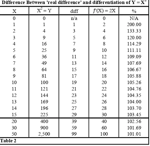
From the theoretical explanations above it must be understood that the derivative does not measure exact change except for a linear function, for any polynomial with a degree 2 or higher the derivative is not accurate. Table 1 shows Y = X and the difference, diff, between each x accumulation as well as the derivative. The last column shows the difference in percentage terms of ƒ’(X)/ difference, as can be seen from table 1 ƒ’(X)/ difference in percentage terms is 100%, they are equal, therefore the derivative is equal.

Difference Between 'real difference' and differentiation of Y = X

X X = Y diff ƒ'(X) = 1 %

0 0 n/a 0 N/A

1 1 1 1 100.00

2 2 1 1 100.00

3 3 1 1 100.00

4 4 1 1 100.00

5 5 1 1 100.00

6 6 1 1 100.00

7 7 1 1 100.00

8 8 1 1 100.00

9 9 1 1 100.00

10 10 1 1 100.00 11 11 1 1 100.00 12 12 1 1 100.00 13 13 1 1 100.00 14 14 1 1 100.00 15 15 1 1 100.00

Table 1

Table 1 is as expected from theory, however let us look at table 2 that shows the difference between the derivative and the ‘real difference’ for Y = X2.

Difference Between 'real difference' and differentiation of Y = X2

X X2 = Y diff ƒ'(X) = 2X %

0 0 n/a 0 N/A

1 1 1 2 200.00

2 4 3 4 133.33

3 9 5 6 120.00

4 16 7 8 114.29

5 25 9 10 111.11

6 36 11 12 109.09

7 49 13 14 107.69

8 64 15 16 106.67

9 81 17 18 105.88

10 100 19 20 105.26

11 121 21 22 104.76

12 144 23 24 104.35

13 169 25 26 104.00

14 196 27 28 103.70

15 225 29 30 103.45

20 400 39 40 102.56

30 900 59 60 101.69

50 2,500 99 100 101.01

Table 2

expected in ratio terms the derivative gets closer to the ‘real difference’, though in the case of Y = X2, the derivative is always 1 greater than the ‘real difference’.

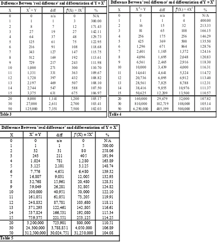
Tables 3, 4, and 5 illustrate the real difference and the derivative for Y = X3, Y = X4, and Y = X5

respectively. As can be seen from tables, 3, 4, and 5, the derivative always higher than the real difference, however the ratio of the difference falls as X, or the independent variable increases. This would be a real problem for example if one is using the derivative to illustrate the marginal revenue.

Difference Between 'real difference' and differentiation of Y = X3

X X3 = Y diff ƒ'(X) = 3X2 %

0 0 n/a 0 N/A

1 1 1 3 300.00

2 8 7 12 171.43

3 27 19 27 142.11

4 64 37 48 129.73

5 125 61 75 122.95

6 216 91 108 118.68

7 343 127 147 115.75

8 512 169 192 113.61

9 729 217 243 111.98

10 1,000 271 300 110.70

11 1,331 331 363 109.67

12 1,728 397 432 108.82

13 2,197 469 507 108.10

14 2,744 547 588 107.50

15 3,375 631 675 106.97

20 8,000 1,141 1,200 105.17

30 27,000 2,611 2,700 103.41

50 125,000 7,351 7,500 102.03

Table 3

Difference Between 'real difference' and differentiation of Y = X4

X X4 = Y diff ƒ'(X) = 4X3 %

0 0 n/a 0 N/A

1 1 1 4 400.00

2 16 15 32 213.33

3 81 65 108 166.15

4 256 175 256 146.29

5 625 369 500 135.50

6 1,296 671 864 128.76

7 2,401 1,105 1,372 124.16

8 4,096 1,695 2,048 120.83

9 6,561 2,465 2,916 118.30

10 10,000 3,439 4,000 116.31

11 14,641 4,641 5,324 114.72

12 20,736 6,095 6,912 113.40

13 28,561 7,825 8,788 112.31

14 38,416 9,855 10,976 111.37

15 50,625 12,209 13,500 110.57

20 160,000 29,679 32,000 107.82 30 810,000 102,719 108,000 105.14 50 6,250,000 485,199 500,000 103.05

Table 4

Difference Between 'real difference' and differentiation of Y = X5

X X5 = Y diff ƒ'(X) = 5X4 %

0 0 n/a 0 N/A

1 1 1 5 500.00

2 32 31 80 258.06

3 243 211 405 191.94

4 1,024 781 1,280 163.89

5 3,125 2,101 3,125 148.74

6 7,776 4,651 6,480 139.32

7 16,807 9,031 12,005 132.93

8 32,768 15,961 20,480 128.31

9 59,049 26,281 32,805 124.82

10 100,000 40,951 50,000 122.10

11 161,051 61,051 73,205 119.91

12 248,832 87,781 103,680 118.11

13 371,293 122,461 142,805 116.61

14 537,824 166,531 192,080 115.34

15 759,375 221,551 253,125 114.25

20 3,200,000 723,901 800,000 110.51 30 24,300,000 3,788,851 4,050,000 106.89 50 312,500,000 30,024,751 31,250,000 104.08

Table 5

Now that a theory has been established as to why the derivative is always higher, a theory and real prove, the prove being in tables 1 – 5, it is time to correct the mistake and look for a new derivative function that will suite our needs for precision and accuracy.

To find the accurate differential we must find the function that will define ƒ’(X) – real difference (diff)

ƒ’k = ƒ’(X) – diff (3)

We can build a general formulae step by step, but first we need to understand why there is a difference between the derivative and the real change, a more compelling reason than merely the tangent, because that will not allow us to extract a real derivative. Take a polynomial say of degree 3, say the function Y = X3. X3 = X · X ·X. Therefore Y = X3 has properties of Y = X2 and Y = X2 in turn has properties that influence it from X. These properties need to be taken out because they are included in the derivative. The larger the polynomial function the more amplified are these properties that need to be taken out. We need to sort of distill the derivative in order to arrive at the real difference, to distill implies purify. In the case of Y = X3, we need to get rid of the properties from the derivative that defines Y = X2 and Y =X.

One can see this effect if one looks at tables 1 – 5 and by how much percentage points, by how high the ratio is that defines derivative over the real difference. When X = 1, Y = 1, and the derivative is 100% in table 1, 200% in table 2, 300% in table 3, 400% in table 4, and 500% in table 5. Table 1, is when X1, table 2, X2, table 3, X3, table 4, X4 and table 5, X5. One can see the influence gets larger and larger, it is this influence that must be removed, this residual influence of Y = Xn, and the residual influence is equal to Y = Xn-1 as well as the influence of ∑(Xn-2→X1). Obviously the greatest influence would be the preceding polynomial. ∑(Xn-2→ X1) is the residual effect of all the other preceding polynomials without including the immediate preceding polynomial, X1 = X.

Knowing what causes the difference between the derivative and the real derivative we can then attempt to build a general formula for the rate of change, in polynomials, but the conclusions will be universal, for all derivatives. Let us look at Y = X2.

Correcting the derivative of Y = X2 should be a fairly simple affair as the only effect that has to be taken out will be the effect of Y = X. Looking at table 1, we look for the pattern that defines the difference between the derivative and the real difference, we see that it is 1, the derivative of Y = X, that also happens to be the real difference. Therefore the rate of change for Y = X2 the real derivative, ƒ’k is:

ƒ’k(X) = ƒ’(X) – ƒ’k(Xn-1) - R (4)

where R is defined as the residual created by ∑(Xn-2→ X)

in this case Xn-2 = 0 and X is already included. Therefore equation (4) becomes

ƒ’k(X) = 2X – 1 (5)

Equation (4) can be the general formula, but it is better to make it look more simple. Not that for Y = X2, the real difference is just the derivative minus 1. That 1 is the real change of Y = X.

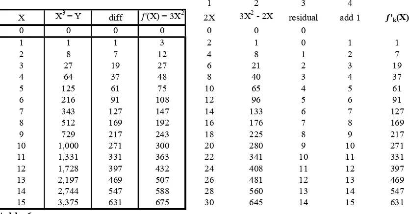
It becomes more complex when we move up to the real change of Y = X3. How do we get the real change, the real derivative. We have a guide in equation (4) Therefore we know that:

ƒ’k(X) = ƒ’(X) – ƒ’k(Xn-1) – R that leads to ƒ’k(X) = 3X2 – 2X – R where

3X2 = ƒ’(X) and

2X = ƒ’k(Xn-1) from equation (5)

Now we need to find R the function that defines the residual effects of all the other residual effects.

1 2 3 4

X X3 = Y diff ƒ'(X) = 3X2 2X 3X2 - 2X residual add 1 ƒ'k(X)

0 0 0 0 0 0 0

1 1 1 3 2 1 0 1 1

2 8 7 12 4 8 1 2 7

3 27 19 27 6 21 2 3 19

4 64 37 48 8 40 3 4 37

5 125 61 75 10 65 4 5 61

6 216 91 108 12 96 5 6 91

7 343 127 147 14 133 6 7 127

8 512 169 192 16 176 7 8 169

9 729 217 243 18 225 8 9 217

10 1,000 271 300 20 280 9 10 271

11 1,331 331 363 22 341 10 11 331

12 1,728 397 432 24 408 11 12 397

13 2,197 469 507 26 481 12 13 469

14 2,744 547 588 28 560 13 14 547

15 3,375 631 675 30 645 14 15 631

table 6

As mentioned above we first must subtract 2X from 3X2 and we arrive at what is the residual. This is under 3 in table 6. Trying to make sense of the residual we see from table 6 that the residual is 1 less than X. To get a function of the residual one will find that to create a function divisible by X one must always add 1 or subtract 1, in all polynomial functions by taking this action one will find the residual will then be divided by X. Adding 1 to the residual we get X. Therefore when Y = X3, the residual is:

R = (X – 1)

Therefore taking our guide from equation (4) we get ƒ’k(X) = ƒ’(X) – ƒ’k(Xn-1) – R (4)

ƒ’k(X) = 3X2 -2X – (X – 1) (6)

we have to subtract 1 from X because we added 1 in table six in order to get the X in the first place. From equation 6 we get the real derivative for Y = X3:

ƒ’k(X) = 3X2 – 2X – X + 1 and by simplification we get

ƒ’k(X) = 3X2 – 3X + 1 (7)

We can test it out to be sure, we can take X = 7 and we get 3(72) – 3(7) + 1

= 147 – 21 +1 = 127 and it is dead on. At one it equals 1.

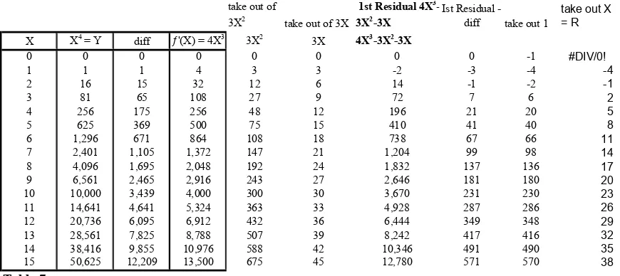
To clarify our understanding let us take one more example, let us take the polynomial Y = X4.We take guidance from equation (4).

ƒ’k(X) = ƒ’(X) – ƒ’k(Xn-1) – R (4)

Therefore when Y = X4 the real rate of change would be ƒ’k(X) = 4X3 - 3X2 – 3X – R. where

4X3 = ƒ’(X)

3X2 – 3X = ƒ’k(Xn-1)

We now will need to solve for R.

Solving for R, that is to say to see the function that defines the residual we shall take the same route as above, the same route as was used to solve for R to find the real rate of change for Y = X3, the ƒ’k (X3). The

process is made easy to understand by including a table to show each step by step process. We include table 7.

take out of

3X2 take out of 3X

1st Residual 4X3 -3X2-3X

Ist Residual - diff take out 1

take out X = R

X X4 _{= Y}

diff ƒ'(X) = 4X3 _3X2

3X 4X3-3X2-3X

0 0 0 0 0 0 0 0 -1 #DIV/0!

1 1 1 4 3 3 -2 -3 -4 -4

2 16 15 32 12 6 14 -1 -2 -1

3 81 65 108 27 9 72 7 6 2

4 256 175 256 48 12 196 21 20 5

5 625 369 500 75 15 410 41 40 8

6 1,296 671 864 108 18 738 67 66 11

7 2,401 1,105 1,372 147 21 1,204 99 98 14

8 4,096 1,695 2,048 192 24 1,832 137 136 17

9 6,561 2,465 2,916 243 27 2,646 181 180 20

10 10,000 3,439 4,000 300 30 3,670 231 230 23

11 14,641 4,641 5,324 363 33 4,928 287 286 26

12 20,736 6,095 6,912 432 36 6,444 349 348 29

13 28,561 7,825 8,788 507 39 8,242 417 416 32

14 38,416 9,855 10,976 588 42 10,346 491 490 35

15 50,625 12,209 13,500 675 45 12,780 571 570 38

Table 7

Having arrived at the known solution of 4X3 – 3X2 – 3X we subtract the difference from the original table 4 and we arrive at what is called the 1st residual - diff. The diff being the real difference. Arriving at the solution we subtract 1. As mentioned above at this stage we must always add or subtract 1 in order to have a function that is related to X. At this stage after adding one we find that R at X = 15 is 570 and at say 3 is 6. After taking out 1 we find we can divide by X. The remaining solution follows the function 3X – 7, therefore R for Y = X4 is:

(3X – 7)X + 1. This can be simplified to: 3X2 – 7X + 1

Taking guidance from equation (4)

ƒ’k(X) = ƒ’(X) – ƒ’k(Xn-1) – R (4) we get

ƒ’k(X) = 4X3 – 3X2 – 3X – (3X2 – 7X + 1), this can be simplified to:

ƒ’k(X) = 4X3 – 3X2 – 3X – 3X2 + 7X – 1 further simplification:

ƒ’k(X) = 4X3 – 6X2 + 4X – 1 (8)

To get real change for Y = X5 the ƒ’k(X) taking guidance from above we get

ƒ’k(X) = 5X4 – 4X3 – 6X2 + 4X – R

and we solve for R, not forgetting to add or subtract 1 before solving for R.

6.3 Conclusion

The derivative is not an accurate measure of the rate of change, it over estimates. Take a Revenue function of the form Y = X4. When we increase from 8 units to 9 units the derivative ƒ’(X) = 4X3 would suggest that additional revenue will equal 243, the reality is that it would be 217, and the ƒ’k (X) would be right and the

derivative would have over estimated.

But it is a simple matter:

ƒ’k = Xin –Xni-1 (9)

for example for a function Y = X7 at 4 the real change = ƒ’k = 47 – 37 = 14 197

In many instances one would however have to solve for R as set out in equation (4), it’s the age of computers it is easier than Newton’s time.

Reference: