Optimal Monetary Policy with Non Zero Net Foreign Wealth

Munich Personal RePEc Archive

Optimal Monetary Policy with Non-Zero

Net Foreign Wealth

Mykhaylova, Olena

University of Richmond, VA

1 July 2010

Online at

https://mpra.ub.uni-muenchen.de/23598/

Optimal Monetary Policy with Non-Zero Net Foreign

Wealth

Olena Mykhaylova

University of Richmond, VA

June 30, 2010

Abstract

I study the impact of net foreign wealth on the optimal monetary policy of an open economy in a two-country DSGE model with incomplete markets, sticky prices and deviations from the Law of One Price. I …nd that by optimally manipulating monetary policy, central banks can a¤ect the timing of interest receipts (or payments) and therefore increase the risk-sharing role of the internationally traded asset. In particular, debtor nations …nd it optimal to allow their currency to ‡oat relatively more freely than do creditor nations. In order to maximize consumer welfare, in most speci…cations of the model central bank should target a weighted average of CPI in‡ation and changes in the nominal exchange rate.

Key words: optimal monetary policy, welfare, open economy, net foreign wealth. JEL classi…cation: E44, E52, F32, F34

1

Introduction

Interaction between exchange rates and the choice of monetary policy rules has been the focus of a multitude of papers in the open economy macro literature1_{. Recent developments in the}

global …nancial ‡ows (currency crises of the late 1990’s, rapid accumulation of U.S. government debt by East Asian countries, and the …nancial crisis of 2008) have also sparked interest in the choice of optimal monetary policy regime for developing countries. Calvo and Reinhart (2002) have documented the fact that many emerging economies exhibit "fear of ‡oating," insofar as their exchange rates, quite independently of the o¢cial stance of the central banks, appear to ‡uctuate within a very narrow band. This observation has motivated many economists to study the question of whether exchange rate targeting could be an optimal policy choice for emerging markets.

This paper utilizes a standard two-country DSGE modeling framework to assess the importance of exchange rate targeting for developing economies, which are characterized by an exogenous interest rate premium on their liabilities (denominated in foreign currency) and non-zero net foreign wealth (NFW) holdings in the steady state. I abstract from the issues of central bank credibility and from any e¤ects of the form of monetary rules on the risk premium. The central question addressed is the choice of monetary policy that maximizes welfare of the emerging economy, given its structural features, the behavior of the foreign country, and exogenous disturbances.

1_{A non-exhaustive list of papers includes Cova and Søndergaard (2004), De Paoli (2009), Devereux (2004),}

The fact that strict in‡ation targeting is optimal only under a very restrictive set of parame-ters has been well-documented in the literature2_{. Moreover, the majority of recent papers analyze}

monetary policy in the framework of a small open economy, a setup that carries with it two impor-tant implications: that the real exchange rate is consimpor-tant because consumption baskets of the two economies (home country and the rest of the world) are identical, and that foreign country is unaf-fected by the choice of monetary rule of the small economy. Therefore, the (often clear-cut) results of these papers may not be valid in a more realistic case of a small country having non-negligible impact on its trading partner.

In many papers cited above, the approach to answering the question of optimal monetary policy has been to rank the following three rules in terms of their implications for welfare and economic stability: CPI in‡ation targeting, PPI in‡ation targeting, and exchange rate peg. I extend the analysis by including "hybrid" policies that target a weighted average of in‡ation and exchange rates. After calibrating the model based on a consensual set of parameter values, I obtain results that are quite di¤erent from the conventional wisdom in the literature that the policy of CPI in‡ation targeting welfare-dominates other options.

I show that the central bank can exploit the risk-sharing value of international assets (more speci…cally, the degree of cyclicality of interest payments or receipts) by adjusting its monetary policy stance in response to the level of NFW. Thus, indebted countries can increase their interest payments to foreigners in good times (following, for example, a local productivity shock) by allow-ing for a sharper depreciation of their currency; analogously, net creditor countries optimally put relatively more weight on exchange rate targeting to reduce capital in‡ows when domestic marginal utility is already low. These results may partly be driven by the relative importance of various disturbances in the calibration: technology shocks tend to dominate the New-Keynesian models3_.

The conclusions of this paper, however, are robust to the inclusion of other common sources of uncertainty (government and demand shocks).

The results of this paper add to the current debate on the optimal monetary policy in the open economy setting. Studies like Obstfeld and Rogo¤ (1995, 2002) have sparked interest in the ability and advisability of monetary policy in‡uencing exchange rates in the context of fully articulated DSGE models. Galí and Monacelli (2005) lay out the theoretical framework to analyze the choice of monetary policy for a small open economy and present a special case for which domestic in‡ation targeting constitutes the optimal regime. Cova and Søndergaard (2004), Benigno and Benigno (2003), and Faia and Monacelli (2008), among others, contemplate the terms of trade channel through which monetary policy can increase welfare of its domestic residents.

The rest of the paper is organized as follows. Section 2 introduces the model and discusses the monetary policy rules under consideration. Section 3 presents the values, used in simulations, of the model parameters and discusses the implications associated with particular choices of these values for the results of the paper. Section 4 analyzes the impact of non-zero steady-state international debt on the choice of welfare-maximizing policy rules. Section 5 summarizes the …ndings and lists several extensions for future research.

2

The Model

The model belongs to the class of DSGE models that are commonly used for evaluating e¤ects of di¤erent monetary policies in both closed and open economy settings.

The model is composed of two countries, home (H)and foreign (F). Both countries are pop-ulated by in…nitely lived households of measure M in the home country and M in the foreign4_;

there is no migration. Households consume all varieties of home and foreign goods and have access to international markets where they can trade a nominal bond. Each country has measure one of …rms that use country-speci…c labor and capital to produce a continuum of domestic goods, which are then traded internationally. Firms are monopolistically competitive, and the prices they set for their products are sticky à la Calvo (1983). International goods markets are segmented because …rms set prices in local currency; therefore, the Law of One Price (LoOP) fails.

The key features of the model are (1) the requirement that foreign liabilities of Home (developing) country are denominated in foreign currency; (2) non-zero steady state NFW of the two countries; and (3) local currency pricing.

The …rst two assumptions are driven by the data. Local currency pricing (which results in incomplete exchange rate pass-through) is motivated by two observations. On the empirical side, the LoOP has been shown to fail when applied to tradable goods (for example, Rogo¤ (1996)); on the theoretical side, it adds another channel through which the central bank can a¤ect the real exchange rate and, consequently, relative consumptions of the two countries (see section 4.1 for details.)

For modeling simplicity, I assume that all goods are traded. As a matter of notation, subscripts

H and F will refer to a good’s country of origin; asterisks will indicate that it is consumed in country F. For example, CH denotes consumption of country H’s good in country F. The two

economies have a similar structure; therefore, most of the equations will be presented only for the Home country.

2.1

Firms

Each country has a continuum of …rms indexed byf on the unit interval. At time t, each Home …rm rents capitalKt 1(f)from the domestic households at the rateRt, hires a labor bundleNt(f)

at the rate Wt and produces one of the varieties of the domestic good. Each …rm is free to set

its own price levelPH;t(f) (denominated in local currency) at home andPH;t(f)(denominated in

foreign currency) abroad.

Home …rms use the following CRS technology to produce output:

Ys

H;t(f) =ZtKt 1(f) Nt(f)1 ;

where0< <1, and Ztdenotes the level of productivity enjoyed by all the home …rms at timet.

Productivity in the two countries evolves according to the following autoregressive process:

lnZt

lnZt

= A11 A12

A21 A22

lnZt 1

lnZt 1

+ "z;t

"z;t

All goods varieties are then bundled into a composite home and foreign goods using the Dixit-Stiglitz

aggregator:

YH;ts =

Z 1

0

YH;ts (f)

1 df

1

where >1. This composite good can then be used for public and private consumption or private investment.

Imposing the zero-pro…t condition, the Home and Foreign prices of the bundle are given by

PH;t =hR

1

0 PH;t(f) 1 _dfi

1 1

and P_H;t =hR₀1P_H;t(f)1 _dfi 1 1

, and therefore aggregate demand

(from consumers, investors and governments) for …rm f’s product is Yd H;t(f) =

h

PH;t(f)

PH;t

i

YH;t

andY d H;t(f) =

h_P

H;t(f)

PH;t

i

YH;t.

As in Calvo (1983), home and foreign …rms reset their prices each period with a constant probability(1 )and(1 ), respectively; otherwise, the old prices remain in e¤ect. If a (home) …rmf gets to announce a new price in period t, it chooses P~H;t(f) and P~H;t(f)to maximize its

expected discounted future pro…ts

Et 1

X

j=t

t;j j t

n

~

PH;t(f)YH;jd (f) +SjP~H;t(f)YH;jd(f) T Cj YH;jd (f) +YH;jd(f)

o

t;j is the home households’ stochastic discount factor: t;j = j t( j_t), where t is the marginal

utility of nominal wealth (de…ned in section 2.2). Notice that in equilibrium,Yd

H;j(f) +YH;jd(f) =

Ys H;t(f).

The optimal prices are given by

~

PH;t =

1

Et

P1

j=t( )j t jPH;jYH;jM Cj

EtP 1

j=t( )j t jPH;jYH;j

~

PH;t = ₁

EtP 1

j=t( )j t jPH;jYH;jM Cj

EtP 1

j=t( )j t jPH;jYH;jSj

and the nominal marginal cost of production is

M Ct=

RtWt1

Zt (1 )1

Notice that in the presence of price stickiness, Home …rms optimally take into account the entire path of future expected nominal exchange rates St when setting foreign prices for their products;

the LOOP need not hold.

I consider a symmetric equilibrium in which every …rm that gets a chance to reset its prices in periodtwill set it to the same value; therefore, optimal prices are not denoted by a …rm subscript (f). As !0and prices become perfectly ‡exible, each period …rms set two new prices

~

PH;t=StP~H;t!'pM CH;t:

Given the price-setting behavior of individual …rms, the aggregate price indices of the Home goods at home and abroad can be written as

P_H;t1 = (1 ) ~P_H;t1 + P_H;t1 ₁

P_H;t(1 ) = (1 ) ~P_H;t(1 )+ P_H;t(1 ₁)

2.2

Households

There is a continuum of households in the home country, indexed by i on the interval [0; M]. A representative household maximizes expected lifetime utility5

Ut(h) =Et 1

X

j=t

j t Cj(h)1

1

Lj(h)1+

1 + (1)

HereCt(h)denotes the household’s consumption of the composite good, which is aggregated from

home and foreign goods using the CES aggregator:

Ct(h) =

1

t CH;t(h)

1

+ (1 t)

1

CF;t(h)

1 1

, (2)

where is the elasticity of substitution between home and foreign goods, and0< t<1determines

the degree of home bias in consumption. Ct(h)denotes consumption of the aggregate good (with

a di¤erent home bias _t) in the foreign country.

The speci…cation of consumption aggregator (2) breaks away from the standard simpli…cation in the open economy literature of equating relative country size and share of domestic good in the consumption basket (i.e., the assumption that small countries consume mostly imported goods) for several reasons. On the empirical side, home bias in consumption has been well documented in the trade literature (for example, Obstfeld and Rogo¤ (2000)). Moreover, by allowing for a di¤erent composition of Home and Foreign baskets, I decouple movements in the two countries’ CPI levels and thus introduce richer dynamics of the real exchange rate, which has non-trivial implications for the choice of optimal monetary policy, as discussed in detail in Section 4.1. Finally, introducing a stochastic process for the home bias parameter will allow us to model demand (preference) shocks.

The prices of the two …nal goods, which also represent the countries’ CPIs, are given by

Pt =

h

tP

1

H;t + (1 t)P

1

F;t

i 1

1

(3a)

P_t = h _tP_F;t(1 )+ (1 _t)P_H;t(1 )i 1 1

(3b)

Consequently, the household (h)’s demands for the composite goods are given by Cd

H;t(h) =

t

h

PH;t

Pt

i

Ct(h)andCF;td (h) = (1 t)

h

PF;t

Pt

i

Ct(h).

5_{Following Woodford (2003), Chapter 3, I model monetary policy as directly targeting (some measure of) in‡ation,}

Households supply di¤erentiated labor services to all the …rms in their country. The composite labor bundle used in production by any given home …rm is given by6

Nt(f) =M

1 1

"Z M

0

Lt(h; f)

1 dh

# ₁

Each household enjoys a degree of monopolistic power in setting its wage Wt(h). The demand

for household(h)’s labor services given its wage is

Lt(h) =

Wt(h)

Wt

Nt

M (4)

HereNt=

R1

0 Nt(f)df is the aggregate demand for the household’s labor services from all …rms in

the economy, andWtis the aggregate real wage: Wt=M

1 1hRM

0 Wt(h)1 dh

i 1

1

. Each household faces the following budget constraint:

Et[ t;t+1Dt(h)] +Btd(h) +StAt(h) +Pt[Ct(h) +It(h) Tt(h)] = (5)

=Wt(h)Ldt(h) +Dt 1(h) + (1 +it 1)Bdt 1(h) + 1 +it 1 p(eat 1 1) StAt 1(h)+ RtKt 1(h) + t(h)

The …rst term on the left-hand side is the price of a portfolio of state-contingent bonds traded domestically, andDt 1 is the payo¤ of such portfolio in periodt. Btd(h)represents household’s

de-mand for the riskless one-period nominal domestic government bond7_{. Households receive transfers}

PtTt(h)from their government (which can be negative in the event of lump-sum taxation). t(h)

represent household’s dividend income.

The modeling of incomplete markets is borrowed from Benigno (2009) and Andrés et al (2006). Home households can buy the foreign bondAt(h), but at a di¤erent price than foreign households.

Home consumers’ priceSt 1 +it p eat a 1

1

depends on their position in the international asset market. Here at M₄S_Pt_tA_Yt_t is the ratio of the aggregate real foreign asset holdings by home

consumers to domestic output, a is the steady state level of at, and the parameter p captures

transaction costs8_{. As lenders (a}

t>0), domestic households pay a higher price for the bond, and

as borrowers they must o¤er a rate of return higher than(1 +i_t). The household’s capital accumulation is given by

Kt(h) = (1 )Kt 1(h) +It(h)

1 2

It(h)

Kt 1(h) 2

Kt 1(h) (6)

Here, the investment good It(h) has the same composition as consumption in (2) and controls

the value of capital adjustment costs.

6_{The scaling factor M}11 _{is necessary to maintain the aggregate relationship} Nt = R

1

0 Nt(f)df = M Lt(h).

Together with the expressionKt=M Kt(h)this will ensure that the production function exhibits constant returns to scale. Additionally, in the steady state the aggregate wageW will equal the individual wageW(h).

7_{In the presence of the complete set of Arrow securitiesDt, government bonds are redundant for the purposes of}

risk-sharing; I introduce them to model the dynamics of national debt.

8_{Equilibrium dynamics of a small open economy with incomplete asset markets generally include a random walk}

Households maximize utility (1) subject to the budget constraint (5), labor demand (4) and capital accumulation constraint (6) by choosing wage rate Wt(h), consumption Ct(h), portfolio

holdingsDt(h),Btd(h)andAt(h), and investmentIt(h).

Wages are sticky, and in any given period a household gets to reset its wage with probability (1 !)((1 ! )abroad). The optimal new wage satis…es

~

W_t +1= 1

Et

P1

j=t(! )j tW

( +1)

j N

1+

j

EtP 1

j=t(! )j t jWjNj

Assuming that every household that chooses its wage in periodt sets it to the same new value, I drop the subscript(h)on the optimal wage rule. Similar to the derivations of the aggregate price level given …rms’ …rst-order conditions, the aggregate wage level is given by

Wt1 = (1 !) ~W

1

t +!W

1

t 1

The rest of the …rst order conditions for the household problem are listed in Appendix A.

2.3

The Government

The aim of this paper is to analyze the e¤ects of various monetary policy rules on consumer welfare. I do not address the question of monetary policy cooperation; instead, it is assumed that the central bank of the Foreign country credibly targets domestic CPI in‡ation (so that CP I

t = 0at all times),

and look for the welfare-maximizing rule that can be adopted by the Home monetary authority. The …rst three monetary policy functions we consider (and which are analyzed in most of the related literature) can be generally written as9

it=Xt; forXt2 CP It ; P P It ; st and ! 1

Here CP I

t and P P It denote Home country’s CPI and PPI in‡ations, respectively, and stmeasures

(log) depreciation of the domestic currency. The parameter controls the degree to which each variable is stabilized around the desired target level (of zero). As ! 1, the central bank eliminates all ‡uctuations in either of the two measures of in‡ation, or nominal exchange rates.

Alternatively, the Home central bank can adopt a variation of the Taylor rule commonly used in monetary literature:

it= (1 i)i+ iit 1+ (1 i) $ CP It + (1 $) st (7)

Here i = 1 1 is the steady state level of the interest rate, and $ indicates the relative weight on in‡ation vs. exchange rate targeting. I study a range of values for this parameter: $ 2[0;1]. Section 3 provides more detail on the calibration of the model.

The Home country …scal authority has the following budget constraint:

Bs

t = (1 +it 1)Bts 1+PtGt+PtTt

Per-capita government purchasesGthave the same composition as consumption in (2).

9_{Cova and Søndergaard (2004) report that these three rules are identical to the more standard speci…cations}

CP I t = 0,

P P I

Each government can a¤ect the functioning of its domestic economy through transfers and purchases. I let government purchases be described by an autoregressive process

lnGt= (1 g) lnG+ glnGt 1+"g;t;

and shocks to government purchases are uncorrelated white noise processes10_{. Transfers react to}

the debt-to-GDP ratio to ensure long-run …scal solvency:

lnTt= (1 tr) lnT+ trlnTt 1+ b(lnB lnBt 1)

In the above equations bars denote steady state values of variables.

2.4

Equilibrium

Goods market clearing conditions are described by

YH;t+YH;t = M(CH;t+IH;t+GH;t) +M CH;t+IH;t+GH;t

YF;t+YF;t = M(CF;t+IF;t+GF;t) +M CF;t+IF;t+GF;t

Equilibrium in the asset markets requires that

Z M

0

Dt(h)dh =

Z M

0

D_t(h)dh= 0

Z M

0

Btd(h)dh = M Bts

Z M

0

At(h)dh+

Z M

0 Bd

t (h)dh = M Bts

Equilibrium in the economy is de…ned by these market clearing conditions and the …rst order conditions of the agents, given the form of monetary and …scal policy rules described above.

2.5

Measure of National Welfare

I de…ne the value function that measures national welfare as

Vt= maxEt 1

X

j=t j t

(

M C_j1

1

1 1 + ALj

)

;

where ALj

RM

0 Lj(h)

1+ _{dh measures the aggregate disutility of work. This function will allow}

me to make quanti…able comparisons of consumer welfare across di¤erent speci…cations of the two economies (for example,Vt measures welfare of a ‡exible price economy, andV~tcaptures the case

of sticky prices). In the case of log utility, the di¤erence between the two value functions,

=Vt V~t

can be interpreted as cost, expressed as percent of consumption, of moving away from the ‡exible price speci…cation to (in the above example) the economy with nominal rigidities.

1 0_{Adding government spending shocks moves the economy farther away from the complete markets allocation and}

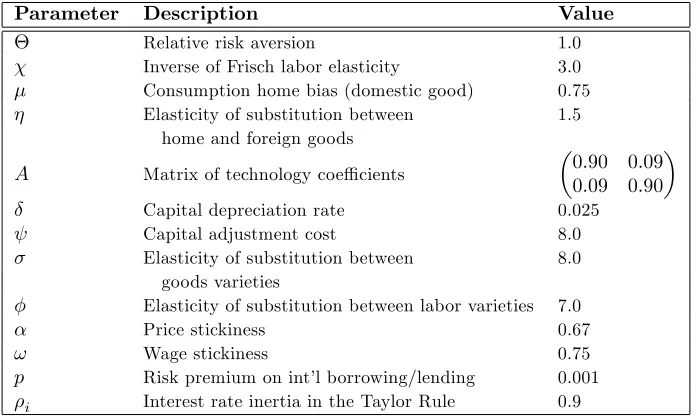
Parameter Description Value

Relative risk aversion 1.0 Inverse of Frisch labor elasticity 3.0 Consumption home bias (domestic good) 0.75 Elasticity of substitution between 1.5

home and foreign goods

A Matrix of technology coe¢cients 0:90 0:09

0:09 0:90

Capital depreciation rate 0.025 Capital adjustment cost 8.0 Elasticity of substitution between 8.0

goods varieties

Elasticity of substitution between labor varieties 7.0 Price stickiness 0.67

! Wage stickiness 0.75

p Risk premium on int’l borrowing/lending 0.001 i Interest rate inertia in the Taylor Rule 0.9

Table 1: Benchmark parameter values

3

Parameterization

Each time period in the model corresponds to one quarter. The benchmark speci…cation is described in Table 1. My goal was to choose the most non-controversial set of parameter values to illustrate the results. Therefore, most of the reported values are standard in the literature; a few others merit further description. Unless otherwise indicated, all parameters describing the Foreign economy are identical to the ones in the Home country.

I assume log utility of consumption, and set = 3, which implies a labor supply elasticity of

1

3. I set = 0:99, which produces a steady state riskless annual return of 4 percent. Cobb-Douglas

parameter in the production function is set to 0.33. Calibration of productivity processes is borrowed from Backus, Kehoe and Kydland (1993), with V ar("z) = V ar("z) = 0:000074, and

Cov("z; "z) = 0:0000185. Elasticities of substitution between goods varieties, , and labor varieties,

, result in price markup of 14 percent and wage markup of 17 percent, respectively.

I follow Canzoneri et al. (2007) in setting the value of nominal price and wage rigidities: = 0:67 and! = 0:75, resulting in price and wage contracts that on average last three and four quarters, respectively.

I set the home bias parameter = 0:75 for all speci…cations of the relative country sizes. However, the parameter must be adjusted as the Foreign country becomes progressively larger, to avoid disproportionate demand on either country’s output; otherwise, discrepancy in steady state unemployment and wages would complicate welfare comparisons11.

There is no agreement in the literature on the appropriate value for the elasticity of substitution between Home and Foreign goods, . However, recent studies report the value of between 1.5 and 2; see Faia and Monacelli (2008) and papers cited therein. I follow Monacelli (2003) in setting this parameter equal to 1.5. The non-trivial implication of this choice of (in conjunction with

1 1_{More speci…cally, the following relationship must hold in all speci…cations of the model:M +M (1 ) =M}

log-utility of consumption) is that Home and Foreign bundles in (2) are substitutes. I perform a robustness check by running the simulations with = 0:9 (complements), and …nd that the conclusions are robust to this change in the parameter value.

The cost of participating in the international asset markets, p, is set to 10 3_{, as in Benigno}

(2009).

3.1

Government Policies

It is a well-known and documented fact that many countries have non-zero net holdings net of foreign assets12_{. In such cases, the policy of producer or consumer price stability may no longer}

be optimal, since nominal exchange rate ‡uctuations may have signi…cant impact on the interest rate spread and the amount of interest paid on international loans.

The ratio of government debt to GDP has to be stationary in the model; …scal policy, therefore, must respond in some way to either de…cit or debt. In the model government transfers respond to the deviation of debt ratio from its steady-state value, which is set at 20 and later 50 percent of GDP13_.

The parameters of the government policy functions are set as follows: _g= _tr = _i = 0:9and

V ar("g) = 0:0082; see Mykhaylova (2009) for details of estimation. Responsiveness of transfers to

the level of debt b was set to 0.1 in order to satisfy the Blanchard-Kahn conditions.

Solution to the model is found using perturbation methods described in Schmitt-Grohé and Uribe (2004) and Collard and Juillard (2001); computer code is written in Dynare (Collard and Juillard (2003)). Second order approximations were used to compute moments, variance decompositions, value functions and impulse response functions presented below.

4

Welfare Results

I consider three di¤erent speci…cations of the relative country size: symmetric case, and Foreign country being four and then nineteen times the size of the Home economy. Recall, however, that in all speci…cations a large portion ( = 0:75) of Home consumer basket consists of domestically produced goods, which makes this analysis di¤erent from the standard small open economy setup. All numbers are reported for the Home country, since the policy of the Foreign central bank is taken to be exogenous.

Before presenting the results of the simulations, it is worth mentioning the mechanisms behind welfare numbers. The …rst two economic ine¢ciencies characterizing the model are nominal rigidi-ties, which lead to ine¢cient allocation of goods produced with the same technology and call for at least some degree of price stabilization, and monopolistic competition, which results in suboptimal levels of output and work e¤ort and introduces an incentive for the central bank to pursue expan-sionary policy. In addition, the failure of the aggregate PPP introduces a channel through which monetary authority can a¤ect domestic consumption by manipulating the real exchange rate and terms of trade.

For each relative size speci…cation, I study the impact of international asset holdings on the welfare-maximizing choice of monetary policy rule. As a benchmark (and for easier comparison with the existing literature), I consider the no-debt steady state, and then discuss welfare implications of non-zero holdings of foreign assets or liabilities on the optimal monetary regime.

4.1

Benchmark Zero-Debt Case

I …nd that in all three size speci…cations, welfare-maximizing policy takes the form of the Taylor rule with a lagged interest-rate term and a weighted average of CPI in‡ation and exchange rate depreciation, as in equation (7).

The …rst (non-controversial) …nding is that adding a lagged interest rate term to the monetary policy rule improves welfare numbers. Thus, pursuing the policy described by it = CP It

1

is welfare-dominated by the rule of the form it = (1 i)i+ iit 1+ (1 i) CP It ; the same

holds true for pure exchange rate targeting. In a forward-looking model, increasing interest rate persistence means that stabilization (of in‡ation, output, exchange rate or any other target of the central bank) requires a much smaller movement of the time-t interest rate, since such movement is expected to prevail far into the future. Lower volatility of interest rates, in turn, implies lower volatility of consumption, output, and labor e¤ort, and thus higher consumer welfare. This result has been discussed in great detail in Woodford (1999), and has also been reported more recently by Senay (2008).

The second result is that the optimal policy in the majority of considered speci…cations is a mix of CPI and exchange rate targeting; more speci…cally, $ in (7) belongs to the open interval (0;1). There are several reasons (documented in literature) why central bank in a New-Keynesian model should pay some attention to the exchange rate movements. As noted in Faia and Monacelli (2008) and De Paoli (2009), the presence of home bias in the international consumption aggregator (2) generates endogenous movements of the real exchange rate in response to the actions of the monetary authority aimed at manipulating terms of trade; real exchange rate, in turn, a¤ects relative consumptions in the two countries14_{. To see this, we substitute (3a) and (3b) into the}

de…nition of the real exchange rateQt St_PP_tt and linearize aroundPH=PF =P andPF;t=PH;t:

qt= [ t+ t 1] t+ t"Ht + t"Ft; (8)

where t pF;t pH;t+st is the terms of trade, and "Ht and "Ft measure deviations from the

LoOP arising due to local currency pricing coupled with nominal rigidities: "F

t pF;t+st pF;t

and"H

t pH;t+st pH;t.

As can be seen from (8), these deviations create an additional channel through which nominal exchange rate can a¤ect consumer welfare (again, through its impact on relative consumptions in the two countries). As discussed in detail in Monacelli (2003), the presence of imperfect exchange rate pass-through calls for an optimal management of nominal exchange rates by the central bank.

4.2

Non-Zero NFW and the Timing of Payments

Having established the fact that some degree of nominal inertia is bene…cial, I now turn to the main question of this paper: the optimal weight on CPI targeting vs. exchange rate targeting in the policy rule of the central bank (the parameter$in (7)). One of the contributions of this work lies in considering the welfare impact of such "hybrid" rules; most of the related literature only considers pure CPI, PPI or exchange rate targeting regimes.

1 4_{International asset markets are incomplete, so the usual link between home and foreign consumption levels,}

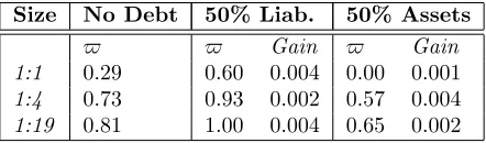
Size No Debt 50% Liab. 50% Assets

$ $ Gain $ Gain

1:1 0.29 0.60 0.004 0.00 0.001

1:4 0.73 0.93 0.002 0.57 0.004

1:19 0.81 1.00 0.004 0.65 0.002

Table 2: Optimal monetary policy ($is the relative weight on CPI targeting in the monetary policy rule),

and welfare gains (measured in percent of consumption), achieved by shifting from the benchmark no debt level of$to its optimal level.

The main results of the simulations are presented in Table 2. The second column shows the optimal (consumer welfare-maximizing) weight on CPI targeting for the three size speci…cations; columns III and V demonstrate how the stance of the monetary policy should be changed when countries accumulate foreign liabilities (in the amount of 50% of their GDP) or foreign assets, respectively. Finally, columns IV and VI show the welfare gain that can be achieved by shifting from the benchmark policy rule (column II) towards the new optimal policy (column III or V, respectively).

Rather provocatively, our welfare calculations suggest that a country that carries a large amount of dollarized foreign debt should pay more attention to targeting CPI in‡ation than a country with no foreign debt. Countries that have large holdings of foreign assets, on the other hand, can maximize their consumers’ welfare by shifting towards exchange rate targeting. This …nding goes contrary to the usual wisdom that it is bene…cial to highly indebted countries to lower their exchange rate volatility and therefore stabilize the value of foreign liabilities. Calvo and Reinhart (2002), for example, present a partial equilibrium model in which the tendency of countries to target the exchange rate is driven by shocks to the international risk premia, an ad-hoc objective function of the central bank that in quadratic in in‡ation deviations, and high pass-through of exchange rates into local prices. This study, in contrast, explicitly models the trade and …nancial interactions of the two economies and encompasses a wider array of disturbances.

Intuition for the results in Table 2 can be gained by considering the risk-sharing service o¤ered by the international asset. Any asset whose payo¤ covaries negatively with consumption o¤ers insurance to Home consumers, and is therefore more desirable15_.

In order to understand how a shift in the monetary policy stance in our model can achieve lower correlation between Home consumption and the payo¤ of the international bond, consider the expression for real income receipts (or payments) on NFW:

Receipts=N F Wt 1 1 +it 1 p eat 1 a 1 St

t

1

Here N F Wt M A_PttSt denotes real NFW of the Home country, expressed in Home consumption

units.

I start by considering the e¤ects of productivity shocks on the Home economy; Graphs 1 and 2 show the impulse response functions of several key variables to this shock for a net creditor country (China, for example) and a net debtor country (Argentina) under di¤erent monetary policy rules. To take advantage of a positive technological shock, which is accompanied by a drop in the Home marginal utility of consumption, a debtor nation (N F W <0) would prefer to temporarily increase

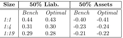
Size 50% Liab. 50% Assets

Bench Optimal Bench Optimal 1:1 0.44 0.43 -0.40 -0.41

1:4 0.31 0.30 -0.23 -0.24

1:19 0.29 0.28 -0.21 -0.22

Table 3: Correlation between Home consumption and debt service for debtor (columns II and III) and creditor (columns IV and V) countries: benchmark (zero-debt) vs. optimal policy.

its interest payments to foreigners. This can be done immediately by allowing a sharp depreciation of the nominal exchange rate, i.e., by shifting the focus of monetary policy away from pegging and towards in‡ation targeting. Conversely, a country with positive holdings of foreign assets (N F W >

0) would prefer to dampen its currency depreciation following an increase in home productivity so as to lower interest income from foreigners when Home marginal utility of consumption is already low16_{. Table 3 o¤ers further evidence in support of this claim: optimally deviating from the}

benchmark policy (of the no-debt scenario) decreases correlation between domestic consumption and debt service for both debtor and creditor nations.

The strength of this channel (which a¤ects the timing of payments and thus enhances the risk-sharing feature of the international bond) depends on the relative importance of the various shocks present in the model. In the next section, I discuss the e¤ects on the optimal policy and consumer welfare of adding a shock to preferences for Home good and increasing the risk premium. The main conclusion, however, remains unchanged: indebted countries tend to bene…t from shifting some of their attention to CPI targeting.

The last thing to note about the results of Table 2 is the increasing preference for in‡ation targeting of small countries (as can be seen in column II, for example). As the Home country becomes progressively smaller, the share of its output in the Foreign country’s consumption, C_t, decreases; consequently, changes in the stance of the Home central bank have an ever-smaller impact on the expected value of foreign consumption, E[C_t]. Through (albeit imperfect) risk-sharing, Home consumption, which is linked to C_t through the real exchange rate, becomes e¤ectively shielded from Home monetary policy. The latter can then be focused more on stabilizing in‡ation, à la the closed-economy setting.

4.3

Other Shocks and Robustness Checks

Welfare gains reported in the previous section, although admittedly very small, represent the lower bound for the true bene…ts from reoptimizing the monetary rule based on net foreign asset position of a country. Most papers studying the question of optimal monetary policy in the open economy setting do not report welfare calculations. Several papers that do perform such calculations report results very similar to ours: welfare gains from optimally adjusting monetary policy are on the order of 0.001-0.01 percent of consumption. See, for example, Benigno (2009), Cova and Søndergaard (2004), and Galí and Monacelli (2005). Below we consider two realistic scenarios that could result in higher welfare gains of reoptimizing monetary policy stance for developing economies than the levels reported in Table 2.

1 6_{While it is di¢cult to distinguish between di¤erent policies by comparing the graphs, close examination of the}

Several related papers have examined the impact of demand shocks on the optimal behavior of central banks in open economy settings. Here we assume that a positive shock increases demand in both countries for Home good (YH) by in‡uencing the home bias coe¢cients:

t = exp(%t); t = =exp(%t)

%t = 0:9%t 1+"%;t

The same adjustment is made to the investment and government spending home biases. Since this shock cannot be measured empirically, its variance was set equal to that of productivity shocks;

E(%) = 0. Adding demand shocks does not change the main conclusion of this paper: debtor nations can increase the welfare of their domestic residents by putting a relatively heavier weight on CPI in‡ation in the Taylor rule of their central banks17_{. Adding this extra source of uncertainty}

doubles the welfare gains relative to those in Table 2.

Developing countries with signi…cant external asset positions often …nd themselves subject to very high interest rate premia, well above our rather conservative 10 basis point spread. For example, Bouvatier (2007) estimates risk premia in several Asian countries to exceed 5 percent during the mid-1990s. Therefore, I repeat the simulations for a higher value of the risk premium,

p= 0:01. Unsurprisingly, welfare gains from optimally adjusting monetary policy increase nearly tenfold.

Put together, these two e¤ects imply that readjusting monetary policy in response to changes in a country’s NFW position could improve consumer welfare by up to 0.1% of steady state consumption.

5

Conclusion

This paper analyzes the impact of non-zero steady-state net foreign wealth on the optimal monetary policy in a dynamic forward-looking model of monetary policy. The utilized framework accounts for the presence of home bias in consumption (which causes deviations from absolute PPP), nom-inal rigidities in price and wage setting, and incomplete international asset markets. I show that international debt changes the welfare-maximizing choice of monetary policy by allowing it to take advantage of the risk-sharing nature of the international bond. The main …nding is that the optimal monetary policy, which is always a mix of CPI and exchange rate targeting, shifts more towards stabilizing in‡ation as countries accumulate foreign debt, and leans closer to pegging in countries that hold foreign assets.

Based on this study, it seems that central banks of developing countries are too concerned with their external position (maintaining the stability of their exchange rate) and are not paying enough attention to internal business cycles (the state of productivity), to the detriment of consumer wel-fare. However, this model is not well suited to understand such a preference for external stability since it assumes away the link between international risk premia, local monetary policy and central bank credibility. Therefore, this study may be missing an additional channel through which ex-change rates a¤ect the behavior of domestic interest rates, output and consumption. In the future work, I hope to pursue this question further by endogenizing the risk premium and studying the impact of policy regime on the behavior of international capital ‡ows.

The model developed in this paper lends itself to several other possible extensions. In order to better understand the interplay of relative country size, NFW position and optimal policy,

1 7_{Naturally, the optimal monetary policy is di¤erent from the case of no demand shocks, but the relative shifts in}

References

[1] Andrés, J., David López-Salido, J., Vallés, J., 2006. Money in an Estimated Business Cycle Model of the Euro Area. Economic Journal 116, 457-477.

[2] Backus, D., Kehoe, P., Kydland, F., 1993. International Business Cycles: Theory vs. Evidence. Federal Reserve Bank of Minneapolis Quarterly Review, Fall 1993.

[3] Benigno, P., 2009. Price Stability with Imperfect Financial Integration. Journal of Money, Credit and Banking 41, 121-149.

[4] Benigno, G., Benigno, P., 2003. Price Stability in Open Economies. Review of Economic Studies 70, 743-764.

[5] Bouvatier, V., 2007. Are International Interest Rate Di¤erentials Driven by the Risk Premium? The Case of Asian Countries. Economics Bulletin, AccessEcon, 5, 1-14.

[6] Calvo, G., 1983. Staggered Prices in a Utility Maximizing Framework. Journal of Monetary Economics 12, 383-398.

[7] Calvo, G., Reinhart, C., 2002. Fear of Floating. The Quarterly Journal of Economics 117, 379-408.

[8] Canzoneri, M., Cumby, R., Diba, B., Mykhaylova, O., 2006. New Keynesian Explanations of Cyclical Movements in Aggregate In‡ation and Regional In‡ation Di¤erentials. Open Economies Review 17, 27-55.

[9] Canzoneri, M., Cumby, R., Diba, B., 2007. The Cost of Nominal Rigidity in NNS Models. Journal of Money, Credit and Banking 39, 1563-1586.

[10] Cochrane, J., 2001. Asset Pricing. Princeton University Press.

[11] Collard, F., Juillard, M., 2001. A Higher-Order Taylor Expansion Approach to Simulation of Stochastic Forward-Looking Models and Application to a Non-Linear Phillips Curve. Compu-tational Economics 17, 125-139.

[12] Collard, F., Juillard, M., 2003. Stochastic Simulations with DYNARE. A Practical Guide. CEPREMAP (http://www.cepremap.cnrs.fr/dynare/).

[13] Cova, P., Søndergaard, J., 2004. When Should Monetary Policy Target the Exchange Rate? Royal Economic Society Annual Conference 2004, No. 51.

[14] De Paoli, B., 2009. Monetary Policy and Welfare in a Small Open Economy. Journal of Inter-national Economics 77, 11-22.

[15] Devereux, M., 2004. Monetary Policy Rules and Exchange Rate Flexibility in a Simple Dynamic General Equilibrium Model. Journal of Macroeconomics 26, 287-308.

[17] Faia, E., Monacelli, T., 2008. Optimal Monetary Policy in a Small Open Economy with Home Bias. Journal of Money, Credit and Banking 40, 721-750.

[18] Galí, J., Monacelli, T., 2005. Monetary Policy and Exchange Rate Volatility in a Small Open Economy. Review of Economic Studies 72, 707-734.

[19] Lane, P., Milesi-Ferretti, G., 2007a. The External Wealth of Nations Mark II: Revised and Extended Estimates of Foreign Assets and Liabilities. Journal of International Economics 73, 223-250.

[20] Lane, P., Milesi-Ferretti, G., 2007b. A Global Perspective on External Positions, in: Clarida R. (Ed.) G7 Current Account Imbalances: Sustainability and Adjustment, The University of Chicago Press: Chicago.

[21] Monacelli, T., 2003. Monetary Policy in a Low Pass-Through Environment. Journal of Money, Credit and Banking 37, 1047-1066.

[22] Mykhaylova, O., 2009. Welfare Implications of Country Size In a Monetary Union. University of Richmond Working Paper.

[23] Obstfeld, M., Rogo¤, K., 1995. Exchange Rate Dynamics Redux. Journal of Political Economy 103, 624-660.

[24] Obstfeld, M., Rogo¤, K., 2000. The Six Major Puzzles in International Macroeconomics: Is There a Common Cause?, in: Bernanke, B., Rogo¤, K. (Eds.), NBER Macroeconomics Annual 2000, Cambridge: MIT Press.

[25] Obstfeld, M., Rogo¤, K., 2002. Global Implications of Self-Oriented National Monetary Rules. The Quarterly Journal of Economics 117, 503-535.

[26] Rogo¤, K., 1996. The Purchasing Power Parity Puzzle. Journal of Economic Literature 34, 647-668.

[27] Schmitt-Grohé, S., Uribe, M., 2004. Solving Dynamic General Equilibrium Models Using a Second-Order Approximation to the Policy Function. Journal of Economic Dynamics and Con-trol 28, 755-775.

[28] Schmitt-Grohé, S., Uribe, M., 2003. Closing Small Open Economy Models. Journal of Interna-tional Economics 61, 163-185.

[29] Senay, O., 2008. Interest Rate Rules and Welfare in Open Economies. Scottish Journal of Political Economy 55, 300-329.

[30] Woodford, M., 1999. Optimal Monetary Policy Inertia. NBER Working Paper No. 7261.

A

Household First Order Conditions

1

Ct Pt

= t

Et t+1 t

= 1

1 +it

1 = Et [1 +it p(eat 1)]

t+1St+1

tSt

tPt = t 1

Ij(h)

Kj 1(h)

t = Etf t+1[(1 k;t+1)Rt+1+ k;t+1 Pt+1] +

t+1

"

(1 ) 1 2

It+1(h) Kt(h)

2

+ It+1(h)

Kt(h)

It+1(h) Kt(h)

# g

0 20 40 60 80 100 0

0.005 0.01

Consumption

L. CPI L. Peg Optimal Bench

0 20 40 60 80 100

-1 0 1x 10

-3 _{Current Account}

0 20 40 60 80 100

0 0.01 0.02

Output

0 20 40 60 80 100

-5 0 5x 10

-4 _{Nominal Interest Rate}

0 20 40 60 80 100

-2 0 2x 10

-3 _{CPI Inflation}

0 20 40 60 80 100

-0.01 0 0.01

Real Exchang e Rate

0 20 40 60 80 100

-5 0 5x 10

-3 _{Terms of Trade}

0 20 40 60 80 100

0.02 0.03 0.04

Net Foreig n Wealth

0 20 40 60 80 100

-5 0 5x 10

-3 _{Chang e in Home/Foreig n Exchang e Rate}

0 20 40 60 80 100

0.02 0.03 0.04

Home Receipts

0 20 40 60 80 100 0

0.01 0.02

Consumption

L. CPI L. Peg Optimal Bench

0 20 40 60 80 100

-2 0 2x 10

-3 _{Current Account}

0 20 40 60 80 100

0 0.01 0.02

Output

0 20 40 60 80 100

-5 0 5x 10

-4 _{Nominal Interest Rate}

0 20 40 60 80 100

-2 0 2x 10

-3 _{CPI Inflation}

0 20 40 60 80 100

-0.01 0 0.01

Real Exchang e Rate

0 20 40 60 80 100

-5 0 5x 10

-3 _{Terms of Trade}

0 20 40 60 80 100

-0.04 -0.02 0

Net Foreig n Wealth

0 20 40 60 80 100

-5 0 5x 10

-3 _{Chang e in Home/Foreig n Exchang e Rate}

0 20 40 60 80 100

-0.04 -0.02 0

Home Receipts