Policy Instruments for Evolution of Bounded Rationality: Application to Climate Energy Problems

(1)

Policy Instruments for Evolution of

Bounded Rationality: Application to

Climate-Energy Problems

Nannen, Volker and van den Bergh, Jeroen C. J. M.

Department of Computer Science, Vrije Universiteit, De Boelelaan

1081a, 1081 HV Amsterdam, the Netherlands, ICREA, Barcelona,

Spain, Department of Economics and Economic History, Universitat

Autònoma de Barcelona, Spain, Institute of Environmental Science

and Technology, Universitat Autònoma de Barcelona, Spain

January 2010

Online at

https://mpra.ub.uni-muenchen.de/43783/

(2)

Policy Instruments for Evolution of Bounded Rationality:

Application to Climate-Energy Problems

Volker Nannen1

Department of Computer Science, Vrije Universiteit, De Boelelaan 1081a, 1081 HV Amsterdam, the Netherlands

J.C.J.M. van den Bergh2

ICREA, Barcelona, Spain

Department of Economics and Economic History, Universitat Autònoma de Barcelona, Edifici Cn, 08193 Bellaterra, Spain Institute of Environmental Science and Technology, Universitat Autònoma de Barcelona, Edifici Cn, 08193 Bellaterra, Spain

Abstract

We demonstrate how an evolutionary agent-based model can be used to evaluate climate policies that take the heterogeneity of strategies of individual agents into account. An essential feature of the model is that the fitness of an economic strategy is determined by the relative welfare of the associated agent as compared to its immediate neighbors in a social network. This enables the study of policies that affect relative positions of individuals. We for-mulate two innovative climate policies, namely a prize, altering directly relative welfare, and advertisement, which influences the social network of interactions. The policies are illustrated using a simple model of global warming where a resource with a negative environmental impact—fossil energy—can be replaced by an environmentally neutral yet less cost-effective alternative, namely renewable energy. It is shown that the general approach enlarges the scope of economic policy analysis.

Keywords: agent-based modeling, behavioral economics, climate policy, evolutionary economics, relative welfare, social network

1. Introduction

The analysis of the economic impact of climate change and climate policy is dominated by neoclassical general equilibrium and growth models. Some models in this vein, which have played a prominent role in the IPCC and international policy debates, are: DICE [1,2], RICE [3], ENTICE [4], CETA [5], MERGE [6] and FUND [7]. Kelly and Kolstad [8] and van den Bergh [9] present brief accounts and evaluations. Although these models have generated many insights, they do not represent the full range of possible approaches nor of the questions that can be ad-dressed. They omit certain elements in their description of reality: out of equilibrium processes, choice between multiple equilibria (path-dependence), structural changes in the economy due to innovations, and the influence of income or welfare distribution on strategies. In addition, the available models assume representative agents, rational behavior, perfect information, and an aggregate production function. This approach allows for exact so-lutions, but it also limits the type of policies that can be studied. For example, they cannot study the effects of information provision, or of exemplary reward and punishment.

Here we present a model that starts from a set of alternative feasible assumptions offered by evolutionary eco-nomics [10,11,12] and by agent-based computational economics [13,14,15]. Evolutionary modeling has gained

Email addresses:[email protected](Volker Nannen),[email protected](J.C.J.M. van den Bergh)

1_{Supported by E.C. NEST Contract n. 018474-2 on "Dynamic Analysis of Physiological Networks" (DAPHNet), Institute for Scientific}

Inter-change, Turin, Italy.

2_{Also affiliated with the Faculty of Economics and Business Administration and the Institute for Environmental Studies, Vrije Universiteit,}

Amsterdam, The Netherlands. Fellow of NAKE and Tinbergen Institute.

(3)

Appli-some popularity in economics, but most studies in this vein lack a policy dimension. This holds especially for applications of pure evolutionary game theory [16]. However, agent-based models applied to economics have rarely addressed public policy issues, and if they have done so, only in a way that does not fully exploit the policy potential offered by an evolutionary model [17]. The present study adds a policy angle to an agent-based evolu-tionary approach, focusing on the opportunities that an evoluevolu-tionary system offers for policy design and analysis. This approach recognizes evolution in the economy rather than emphasizing the use of evolutionary algorithms to optimize non-evolutionary complex systems [e.g.18].

The evolutionary agent-based model developed here addresses policy in a setting of global warming. The lat-ter is endogenous to the model and depends on the source of energy used by agents in the model. These agents may be interpreted as national or regional authorities in charge of the energy policy of an independent economy. Global warming is assumed to have a negative effect on social welfare. The overall goal at the global level is to replace a resource with a negative impact on social welfare—fossil energy—by a neutral alternative, namely re-newable energy. On an individual level the alternative comes with no economic advantage, and possibly even with a disadvantage, so that there is no incentive to adopt it. A complicating factor is that there is no central au-thority that can formulate and enforce a policy. Climate policies are usually based on international agreements, and compliance by countries is voluntary.

Strategic decisions by governments regarding energy investments are normally not taken in solation of what happens in the rest of the world. Here we study mutual influences of experiences of governments/countries with their energy investment strategies. The resulting dynamics can be captured by an evolutionary model of imita-tion. Each agent is modeled individually and agents are assigned only limited information and boundedly ratio-nal capabilities. Their objective is assumed to be to reach a high level of individual welfare. The only informa-tion available to the agents are the investment strategies and the income growth rates of their fellow agents. The agents believe that there is a strong causal link between these two variables. Since they prefer a high over a low income growth rate, they imitate the investment strategy of a fellow agent when that fellow agent realizes an in-come growth rate that is high relative to their own inin-come growth rate and that of their other fellow agents. That is, they imitate an investment strategy when they believe that it causes a relatively high income growth rate. This approach is inspired by findings on relative welfare and income comparison effect of happiness or “subjective well-being” studies [e.g.19,20].

Imitation is never perfect. Small errors are introduced during the imitation process that lead to slightly dif-ferent variants of the same investment strategy. While these errors are necessary to maintain diversity within the pool of strategies and to allow a population of imitating agents to find and converge on the individually optimal strategy, they also form a hitherto unexploited opportunity for the policy maker. If the desirable variant is given a selective advantage over the undesirable variant, the first will diffuse faster and will ultimately be used more often. For example, a policy that aims for agents to adopt a greener investment strategy—in the sense that they invest less in fossil energy—can do so by convincing at least some agents that the greenest variants in the current pool of strategies lead to a relatively high income growth rate. As these strategies are imitated, the errors guaran-tee that some of the new variants will be greener still. An evolutionary policy can thus “breed” a new strategy by progressively giving a selective advantage to the most desirable variants.

As has been extensively discussed by Wilhite [21], agent-based simulation of economic processes needs to give proper attention to the social network. Communication links between economic agents, individuals and institu-tions, are neither regular nor random. They are the result of a development process that is steered by geographic proximity, shared history, ethnic and religious affiliation, common economic interests, and much else. The social networks used for this study reproduce a number of stylized facts that are commonly found in real social networks: the small world effect [22], a high clustering coefficient [23], and a scale-free degree distribution [24]. Modeling the evolution of strategies in such complex social networks allows us to formulate economic policies that exploit the effect of social visibility on the diffusion of a desirable strategy.

(4)

[image:4.595.139.466.126.287.2]

Table 1: Economic and climate variables

a,b individual agents n number of agents in the population

t time step k average number of neighbors per agent

N neighbors of an agent C _{clustering coefficient of the network}

s investment strategy σ mutation variance of strategies F _{fitness of a strategy} _Q _{income without global warming}

Y net domestic income γ income growth rate K general capital sector α Cobb-Douglas exponent F fossil energy sector τ tax on fossil energy investments

δ capital discount rate T _{revenue of the fossil energy tax}

R renewable energy sector c additional cost of renewable energy G greenhouse gas level φ breakdown fraction of greenhouse gas v scale of climatic damage ε environmental tax on income

β scaling factor E _{fund financed by the environmental tax}

a monetary award/reward. The other policy, advertisement, increases the social visibility of exemplary agents by increasing their connectivity in the social network. Policy tools that increase social visibility include, for instance, sponsorship of industrial fairs and scientific venues, and the production and distribution of educative material.

The remainder of this article is organized as follows. Section2presents the climate-economy model, including the evolutionary mechanisms of strategy formation and diffusion, and formulates the climate policies. Section3 studies the convergence behavior of the resulting evolutionary process. Section4evaluates the climate policies using numerical simulations with the climate-economy model. Section5concludes.

2. The economic model

2.1. General features of the model

The present economic model is formulated in order to study the effectiveness of regulatory public policies when economic behavior evolves through social interactions. The approach focuses on climate policies and en-ergy investment strategies, but the model can easily be adapted to other problems. Each agent controls an inde-pendent economy with its own supply and production. The agent formulates a strategy to invest current domestic income in different sectors. The returns for each independent economy are then calculated from standard eco-nomic growth and production functions. Some allocations give higher returns than others, and the goal of the agents is to find a strategy that can realize a high level of individual welfare.

The present model is loosely based on the influential work of W. D. Nordhaus, who published a series of general-equilibrium economic models of climate policy and global warming, starting with the DICE model [25]. From this model all economic factors that were not essential to the current study were removed, in particular elements relating to labor, technical details of global warming, and resource constraints. The reason is that our model aims to be illustrative rather than to accurately replicate reality. Moreover, simplification here allows for additional complexity in the module describing the evolution of strategies.

A fundamental difference between the present evolutionary agent-based approach and the general-equilibrium approach of Nordhaus is that here agents do not make perfectly rational decisions that are based on perfect knowl-edge. Instead, agents evolve their strategies through random mutation and selective imitation in a social network. Moreover, while here agents are homogeneous in terms of production functions, initial strategies and initial in-come, they are heterogeneous in their placement in the social network and the information they receive, and their strategies and income quickly diverge.

(5)

Each policy is evaluated over a period of 400 time steps, simulating 400 quarters or 100 years, a period that is suf-ficiently long to study the long-term effects of a policy on climate and welfare. As no significant financial market requires a publicly traded company to publish financial results more than 4 times a year, we consider a quarter to be the limit of feasibility to account for growth and to review an economic strategy. Given habitual behavior and organizational routines [10], most economic agents will in fact review their strategy less often.

2.2. Strategies, investment, and production

All parameters of the economic model are summarized in Table1. Our basic model of energy investment consists of three investment sectors: general capitalK, fossil energyF, and renewable energyR. Here, the capital accumulation in an energy sector includes technology, infrastructure, and licenses for production, distribution, and consumption of a particular form of energy. LetYa(t) be the income of agenta at timet. Formally, the investment strategysa(t) of an agent can be defined as a three dimensional vector

si,a(t)∈[0, 1] ,

X

i∈{K,F,R}

si,a(t)=1. (1)

The non-negative partial strategysi,a(t) determines the fraction of the previous period’s incomeYa(t−1) that agentainvests in sectori at timet. All partial strategies are constrained to add up to one. The set of all possible investment strategies is a two dimensional simplex (i.e., a triangular surface) embedded in a three dimensional Euclidean space.

Invested capital is non-malleable: once invested it cannot be transferred between sectors. The accumulation of capital in each sector depends on individual investment and the global depreciation rateδ, which is constant and equal for all sectors and all agents. In the case of fossil energy the investment can be reduced by a regulatory taxτon investments in the fossil energy sector. This tax is defined as a fraction of fossil energy investments before taxes, so that a tax ofτ=100% doubles the cost of all expenditures on production, distribution and consumption of fossil energy. In this way, if an agent’s total spending on fossil energy isx=Ya(t−1)sF,a(t), then an amount of

x

1+τis indeed invested, while the remaining xτ

1+τis paid as a tax. The revenue

T₍_t₎= τ 1+τ

X

a

Ya(t−1)sF,a(t) (2)

of this tax is recycled and distributed evenly among all agents.

To model a competitive disadvantage for renewable energy—for example through a higher cost of technology, production, or storage—we introduce an additional costcfor renewable energy, representing the difference be-tween the costs of renewable and fossil energy. In analogy to the fossil energy taxτ, we express this additional cost in percent of the unit cost of fossil energy before taxes, i.e., renewable energy is twice as expensive as fossil energy before taxes whenc=100%. The difference equations for non-aggregate growth per sector are then

∆Ka(t)=Ya(t−1)sK,a(t)−δKa(t−1) (3)

∆Fa(t)= Ya(t−1)sF,a(t)

1+τ −δFa(t−1) (4)

∆Ra(t)= Ya(t−1)sR,a(t)

1+c −δRa(t−1). (5)

We proceed by first calculating the income of agentaas if there had been no global warming, and then by accounting for global warming. We calculateQa(t) from the returns of the individual capital sectors by a Cobb-Douglas type production function with constant returns to scale and constant elasticity of substitution,3

Qa(t)=β£

Ka(t)¤α£

Fa(t)+Ra(t)¤1−α, (6)

3_{Instead of including the fossil energy tax}_τ_{and the additional cost}_c_{of renewable energy in the growth functions, they might be}

incorpo-rated in the production function,

Qa(t)=β[Ka(t)]α ·_F

a(t) 1+τ+

Ra(t) 1+c

(6)

whereβis a scaling factor. In this production function fossil energy and renewable energy are assumed to be perfect substitutes: one can completely replace the other. General capital and combined energy are assumed to be imperfect substitutes. Production requires both types of input, and only a specific combination will lead to a high production level.

Global warming is commonly defined as the increase of global mean temperature above the pre-industrial mean, due to an increased level of atmospheric greenhouse gasesG(t). The dynamics of the greenhouse gas effect include many local and global subsystems, resulting in complex and chaotic dynamics that allow for a range of possible climate scenarios [e.g.,26]. Here we just include a simple feedback loop that captures one of the main characteristics of greenhouse gas induced economic damage: a long delay between action and reaction that spans several decades. We do so by modeling the level of atmospheric greenhouse gases as a result of only two factors: cumulative fossil energy consumption by economic agents, which we assume to be equal to the total amount of capital accumulated in the fossil energy sector, and a natural breakdown fractionφ,

∆G(t)=X

a

Fa(t)−φG(t−1). (7)

We assume that renewable energy does not contribute to global warming. We further pose the relationship be-tween economic damage, global warming, and economic damage to be linear, scaled by a factorv. The net income Ya(t) of an agentacan then be calculated as

Ya(t)=Qa(t) [1−vG(t)]+ T(t−1)

n . (8)

whereT₍_t−1) are the revenues from the regulatory taxτ, distributed with one time step delay among thenagents of the population. The growth rateγa(t) of the income of agentais

γa(t)= Ya(t)

Ya(t−1)−1. (9)

2.3. The social network

To model which agent can imitate which other agent we arrange all agents in a social network where the nodes are agents and the edges are communication links. We use a generic class of social networks that has been well studied and validated in network theory, namely small world networks that have a scale-free degree distribution generated by a stochastic growth process with preferential attachment [24] and that have a high clustering coeffi-cientC_.4

Before the start of each simulation we use a stochastic process to generate a new bi-directional network. The process assigns each agentaa set of peersNathat does not change during the course of the simulation. If agenta is a peer of agentb, thenawill consider the income growth rate and the investment strategy ofbwhen choosing an agent for imitation, whilebwill consider the income growth rate and the investment strategy ofa. On the other hand, ifaandbare not peers, they will not consider each other for the purpose of imitation. The generating process starts from a circular network where each agent has two neighbors—i.e., average connectivityk=2—and iteratively adds new edges to the network until the desired average connectivitykis reached. The agents for the next new edge are chosen at random with a probability that is proportional to their connectivity (hence the term ‘preferential attachment’) and their proximity in the network, i.e., the inverse of the minimum number of links to traverse from one agent to the other.

The random way in which the network is created guarantees that the average distance between any two agents is very short, significantly shorter for example than in a regular grid. The preferential attachment leads to a very skewed distribution of peers per agent, with some agents having several times the median connectivity. These well-connected agents act as information hubs and dominate the flow of information. A high clustering coefficient

4_{In their seminal paper Watts and Strogatz [23] define the clustering coefficient}C_i_{of a node}_i_{as the number of all direct links between}

(7)

implies that if two agents are peers of the same agent, the probability that they are also peers of each other is significantly higher than the probability that two randomly chosen agents are peers. This leads to the emergence of blocks within the social network that exhibit a high level of local interconnectivity, like for example the European Union in the case of independent nations.

2.4. Evolution of strategies

From the point of view of evolutionary modeling, agents and investment strategies are not the same: an agent carries or maintains a strategy, but it can change its strategy and we still consider it to be the same agent [27]. Because every agent has exactly one strategy at a time, the number of active strategies is the same as the number of agents.

At each time step an agent may select one of its peers in the social network and imitate its strategy. If that happens, the strategy of the imitating agent changes, while the strategy of the imitated agent does not. The choice of which agent to imitate is based on relative welfare as indicated by the current growth rate of income. Note that the relation between incomeYa(t) and growthγa(t) is

Ya(t)=Ya(0) t

Y

i=1 £

γa(i)+1

¤

. (10)

The imitating agent always selects the peer with the highest current income growth rate. Only if an agent has no peer with an income growth rate higher than itself, the agent does not revise its strategy.

If imitation were the only mechanism by which agents change their strategies, the strategies of agents that form a connected network must converge on a strategy that was present during the initial setup. However, real imitation is never without errors. Errors are called mutations in evolutionary theory. They are fundamental to an evolutionary process because they create and maintain the diversity on which selection can work. In this model we implement mutation by adding some Gaussian noise to the imitation process. That is, when an agent imitates a strategy, it adds some random noise drawn from a Gaussian distribution with zero mean to each partial strategy. This causes small mutations along each partial strategy to be more likely than large ones. The exact formula by which agentaimitates and then mutates the strategy of agentbis

si,a(t)=si,b(t−1)+N(0,σ). (11)

N_(0,_σ_{) is a normally distributed random value with zero mean and standard deviation}_σ_{, drawn independently} for each dimension. Because partial investment strategies have to sum to one, we have to enforceP

isi,a(t)=1, for example by orthogonal projection of the mutated strategy on the simplex. This constraint effectively removes one degree of freedom from the error term, which becomesN_(0,_σ_{) for each orthogonal axis of the simplex. Imitation is} further constrained to leave all partial strategies positive. If the new strategy falls outside of the simplex, we satisfy this constraint by replacing it with the closest strategy within the simplex. Needless to say that we do not imply that our boundedly rational agents engage consciously in such mathematical exercises. Subjectively they merely allocate their income such that none is left.

In order to measure the impact of an individual agent on the evolution of strategies at the population level, we need to introduce the concept of fitness. In analogy with biology, where fitness usually measures an individual’s capability to reproduce, we define the fitness of an economic agent as the frequency with which it is imitated. In the model that has been presented so far, the frequency with which agenta is imitated is fully determined by the income growth rate ofaand its first and second degree neighbors. Further degrees do not matter. First degree neighbors are relevant because only direct neighbors considerafor imitation. Second degree neighbors are relevant as they are the agents thatacompetes with. Agentawill only be imitated by agentbifahas a higher income growth rate thanband all other neighbors ofb(who are second degree neighbors ofa).

This functional relationship can be expressed by a fitness function. Let {Nb∪b} be the set consisting of agent band its peers, i.e., those agents with which agentbcompares its income growth rate. Letγmax_N

b∪b(t) be the income

growth rate of the fastest growing agent in this set at timet,

γmax_N

b∪b(t)=argmax

c∈{Nb∪b}

(8)

Then the fitnessF_a₍_t_{) of agent}_a_{at time}_t_is

F_a₍_t₎= X

b∈Na

(

1 ifγa(t)=γmax_N

b∪b(t),

0 otherwise. (13)

Or, in set notation:

F_a₍_t₎=¯¯{b|b∈Na∧γ_a(t)=γmax

Nb∪b(t)}

¯

¯. (14)

In this function the fitness of an agent is bounded by the number of its neighbors. An agenta1who has just one neighbor and has the highest income growth rate among the neighbors of that neighbor has a fitness of one, whereas an agenta10who has ten other neighbors and whose income growth rate is highest among the neighbors of just two of them has a fitness of two, even if in absolute termsa1has a much higher income growth rate than

a10. We see that the principal factors that determine the fitness of an agent are relative welfare as indicated by the current growth rate of income as well as the number of agents it communicates with. This gives us two different means by which a policy can regulate the evolution of economic strategies: either by changing the income growth rate of some agents, depending on the desirability of their current strategies, or by changing their connectivity in the social network, again depending on the desirability of their current strategies.

2.5. Policy goals and formulation

The goal of the policies that are being studied here is to let the economic agents reach a high social welfare. Assuming that fossil fuel consumption has a negative economic impact because of the associated global warming, a successful policy has to reduce consumption in fossil fuels but without considerably reducing social welfare, such that the social costs of implementing the policy do not outweight the social benefits from a reduction in global warming.

We will study three policies, starting with a taxτon fossil energy investments. This is the first best policy under traditionally assumed conditions (rational agents, perfect markets), and we study it here in the context of imperfect information and bounded rationality. It is a regulatory and not a revenue raising tax and is defined as a fixed percentage on all investments in fossil energy, cf. equation2,4, and8. We compare this standard policy with two novel policies that take advantage of the evolutionary process by increasing the fitness of those agents that invest a larger fraction of their income in renewable energy. These policies increase the fitness of an agent either by increasing its income growth rate, or by increasing its visibility in the social network. The rationale is that, if we increase the fitness of agents that use certain strategies, these strategies will be employed more frequently.

Under the first policy, agents pay a tax that is proportional to their investment in fossil fuel. This tax makes investment in fossil energy economically less attractive. However, since the incentive not to comply with this policy is also proportional to their investment in fossil fuel, the effect of this policy depends much on the existence of a central authority that can enforce it. The second policy studied here, a prize, increases the fitness of agents that invest a larger fraction of their income in renewable energy by awarding them a monetary prize, financed by a global tax that is paid by all agents. That is, it is not important who pays the tax, as long as someone pays it, for example those agents that are most affected by global warming. This does not entirely solve the problem of compliance, but makes it less acute. The third policy, advertisement, increases the fitness of agents that invest a higher fraction of their income in renewable energy by increasing their social visibility, i.e., their connectivity in the social network. No compliance is required.

The prizes policy gives a monetary prize to those agents who invest the largest fraction of income in renewable energy, increasing their relative welfare, and with that their fitness. This prize is financed by an environmental tax

εon production after damage from global warmingQa(t) [1−vG(t)]. Since this is a revenue raising tax to finance the policy and not a regulatory tax that depends on individual behavior, it has the same level for each agent. Let E₍_t_{) be the size of the environmental fund at time}_t_:

E₍_t₎=X

a

(9)

Table 2: Free policy parameters

Fossil energy tax τ tax on fossil energy investments Prize policy q number of agents that receive the prize

ε tax on income to finance the prize Advertisement policy q number of agents that are advertised

p probability that an agent is reached by advertisement (the simulations use a fixed value ofp=.25)

At each time step, theq agents that invest the highest fraction of their income in renewable energy are each awarded an equal shareE₍_t−1)/q, such that under the prizes policy the net income becomes

Ya(t)=Qa(t) [1−vG(t)] [1−ε]+

(

E₍_t₋_1)/_q _if_a_{is awarded a prize,}

0 otherwise. (16)

To give an example: if the income taxεis 1%, and 10 out of 200 agents are selected to receive a prize, then under the assumption that their income does not deviate significantly from the average income, it is raised by about 20%. If the majority of agents receive a prize, the tax to finance the prize is in effect a selective punishment of those agents that invest relatively much in fossil fuels.

The advertisement policy increases the social visibility of those agents that invest the largest fraction of their income in the renewable energy sector, increasing the number of agents that consider the advertised agents when deciding whom to imitate. At each time step theqagents that invest the largest fraction of their income in re-newables are selected to be advertised. The advertised agents are temporarily added to the group of neighbors of some other agents, so that these other agents consider the advertised agents when deciding whom to imitate. Advertisement does not oblige an agent to consider an advertised agent. Instead, its success rate depends on the resources invested in the campaign. For simplicity we assume that whether agentaconsiders the advertised agent bfor imitation is an independent random event for eacha,bandtand has probabilityp. We ignore the cost of advertisement and assume a success rate of justp=.25.

To give an example, let the average number of neighbors per agent before advertisement bek=10 and letq=8 agents be selected for advertisement. On average, each agent can now choose betweenk+q∗p=10+8∗.25=12 neighbors when deciding whom to imitate. If an agent imitates, chances are one in six that it imitates the strategy of an advertised agent, provided that the income of the advertised agents does not deviate significantly from that of the other agents. The free parameters of each policy are listed in Table2.

2.6. Model calibration

The economic model is simulated in Matlab. This way, basic matrix operations can be used to implement the various difference equations, as well as the imitation process, which depends on the local neighborhood structure of the social network. (A social network can be represented by a boolean matrix with one row and column for each agent, and where the value of each combination of row and column reflects whether a link exists between the respective agents.) The free parameters of the economic model are calibrated such that global warming has a significant negative welfare effect, emphasizing the need for policies. The calibrated values of all free economic parameters are summarized in Table3.

[image:9.595.133.469.682.731.2]

A fixed number 200 of agents is used in all simulations; this is approximately the number of independent states and a rough approximation of the number of agents with an independent energy policy. The quarterly capital

Table 3: Calibrated parameter values of the economic model

k network connectivity 10 C _{clustering coefficient} _.66

σ mutation variance .02 α Cobb-Douglas exponent .9

δ capital discount rate .01 φ breakdown of greenhouse gases .01

(10)

average

income

0 0.01 0.02 0.03 0.04 0.05 0.06 0.07 0.08 0.09 0.1

3.2 3.4 3.6

[image:10.595.131.467.123.205.2]

mutation variance

Figure 1: Effect of the mutation variance on economic performance

discount rate isδ=.01. The exponent of general capital in the production function isα=.9, and the exponent of the combined energy sector is 1−α=.1. In this way income is highest when 90% of an agent’s capital is in the general sector and 10% in the two energy sectors. The scaling factorβof the production function is calibrated such that the calibrated economic model without climate damage has an economic growth rate of about 2% per annum. The breakdown fractionφof greenhouse gas and the sensitivityvto global warming are calibrated such that without any climate policy the greenhouse gas emissions reduce the per annum growth rate by an order of magnitude over the 100 years of the simulation, consistent with the studies reported in Section1.

The mutation varianceσis the only free parameter that regulates the evolutionary mechanism. Small values of

σslow down the discovery of a good strategy. Large values prevent convergence. A good value ofσlies somewhere in between. Figure1shows how the average income of the agents depends onσ. Thex-axis shows different values forσ. They-axis shows the average income that a population of 200 agents realized after 400 time steps. Each measurement point in the graph is averaged over 100 simulations. The initial strategy of each agent is chosen at random. There are no taxes, global warming has no effect, and the additional cost of renewable energy isc= 100%. Under these conditions the optimal strategy that maximizes the income growth rate of an individual agent is〈sK,sF,sR〉 = 〈.9, .1, 0〉. The graph shows that average income is maximized for a value of approximatelyσ≈.02, and for this reason we use a value ofσ=.02 in the remainder of this study.

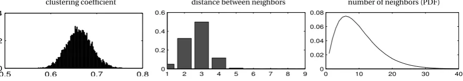
For the social network we use an average connectivity ofk=10. In a population of 200 agents this value re-sults in a highly connected network—the average distance between any two agents in the network is 2.7—while maintaining the overall qualities of a complex social network. Figure2shows some key statistics collected from 10,000 networks of 200 agents that were created by the stochastic growth process using these values: a normal-ized histogram of the clustering coefficientC _{of each network (average}C _{is .66), a normalized histogram of the} distance between any two agents in each network, and the probability density function (PDF) of the number of neighbors per agent in each network. Note the relatively high probability of having 20 or more neighbors when the average connectivity is 10 neighbors. Such significant numbers of highly connected agents do not exist in regular grid networks or random networks of the Erd˝os-Rényi type, yet their existence in real social networks is well estab-lished [28]. They generally act as information or transportation hubs and accelerate the dissemination of goods, viruses and ideas.

In order to avoid any dependency of the simulation results on initial conditions, the numeric simulations are divided into an initialization phase and a main experimental phase. During the initialization phase certain parameters of the evolutionary economy will converge regardless of the initial conditions, contributing to the

clustering coefficient

0.5 0.6 0.7 0.8

0 2 4

distance between neighbors

1 2 3 4 5 6 7 8 9

0 0.2 0.4 0.6

number of neighbors (PDF)

0 10 20 30 40

0 0.02 0.04 0.06 0.08

[image:10.595.69.527.623.703.2]

(11)

allo

cation

0 100 200 300 400 500 600 700 800

0.85 0.9 0.95

general capital

time steps

allo

cation

0 100 200 300 400 500 600 700 800

0 0.05 0.1

fossil energy renewable energy

[image:11.595.126.470.117.304.2]

time steps

Figure 3: Convergence of the average investment strategy

general validity of the numerical results. The initialization effect is visualized in Figure3, which shows how the average investment strategy converges on an equilibrium. 800 time steps are shown. Initial strategies are chosen at random from the two dimensional simplex, and so att=1 the average strategy is〈sK,sF,sR〉 = 〈1_/3,1_/3,1_/3〉. The average strategy att=800 is〈.9, .09, .01〉. Results are averaged over 10,000 simulations.

Note that while it takes the agents only about a dozen time steps to learn to invest some 90% of their invest-ments in general capital, they need about 200 time steps to become sufficiently sensitive to the difference in cost between the two energy sectors and to differentiate their energy investments. Fromt=200 tot=400 the con-vergence on the final strategy can be seen to follow a damped oscillation pattern. The full effect of a policy can only be established if it is introduced after the system without policy has reached equilibrium. It takes 400 time steps for the system without a policy to converge, and so we base the numeric evaluation of climate policies on simulations that consist of an initialization phase of 400 time steps during which no policies are applied, followed by a main experimental phase of 400 time steps during which policies are applied and evaluated. In particular, the taxτon fossil energy investments and the environmental taxεare always zero up untilt=400. Only fromt=401 they take the value assigned to them by the respective policy.

3. The evolutionary dynamics

3.1. Derivation of the growth function

An important prerequisite for regulating an evolutionary system is to understand its dynamics. Here we are primarily interested in what strategy the agents will converge on. With regard to global warming we are further interested in whether the evolutionary agents can converge on a globally optimal strategy, rather than on individ-ually optimal strategies.

While the fitness function describes how the imitation of a strategy (the genotype) depends on welfare as in-dicated by the income growth rate (the phenotype), thegrowth functiondescribes how a strategy determines the income growth rate of the agent that carries it. The growth function calculates the economic utility of a strategy as the equilibrium growth rate to which the income growth rate of an agent converges if it holds on to that particular strategy. Derivation of the growth function is essential for an understanding of the evolutionary dynamics. We will base it on an analysis of the ratio of sector specific capital to income.

To start with, equation4and5can be combined to express the difference equation of a combined energy sectorE=F+R,

∆Ea(t)=Ya(t−1)

µ

sF,a(t) 1+τ +

sR,a(t) 1+c

¶

(12)

where the combined energy investment strategy of an agent issF,a(t)+sR,a(t)=1−sK,a(t). Letra(t) be the fraction of 1−sK,a(t) that is invested in fossil energy, and 1−ra(t) the fraction that is invested in renewable energy,

ra(t)= sF,a(t) 1−sK,a(t)

. (18)

This enables us to rewrite equation17as

∆Ea(t)=Ya(t−1)£

1−sK,a(t)

¤

f(ra,t)−δEa(t−1), (19)

wheref(ra,t) stands for

f(ra,t)= ra(t) 1+τ+

1−ra(t)

1+c . (20)

We collapse the scaling factor and the economic effect of global warming into a single factorζ(t),

ζ(t)=β[1−vG(t)] . (21)

Next we combine the calculation of income (equation8) with the production function (equation6) and simplify it by ignoring the additive termT(t_n−1), which is identical for all agents,

Ya(t)=ζ(t)Ka(t)αEa(t)1−α. (22)

We now use equation3and9to calculate the difference equation of the ratio of general capital to income as

Ka(t) Ya(t)=

Ya(t−1)sK,a(t)+(1−δ)Ka(t−1) (γa(t)+1)Ya(t−1)

= sK,a(t)

γa(t)+1

+ 1−δ

γa(t)+1

Ka(t−1) Ya(t−1).

(23)

This dynamic equation is of the form

x(t)=a+bx(t−1), (24)

which under the condition 0≤b<1 converges monotonically to its unique stable equilibrium at

lim

t→∞x(t)=a/(1−b). (25)

In a model without global warming this condition is normally fulfilled: investment is always non-negative and sector specific capital cannot decrease faster thanδ. Theoretically, excessive economic damage caused by global warming allows for economic decline that exceeds the capital discount rate, i.e.,γa≤ −δ. However, the social and political ramifications of such a catastrophic decline are beyond the scope of this model. Hence, with the restriction that this model only covers the caseγa> −δ, and considering that 0<δ≤1, we have the required constraint for convergence

0≤ 1−δ

γa(t)+1

<1. (26)

We conclude that the ratio of general capital to income converges to

lim t→∞

Ka(t) Ya(t)=tlim→∞

sK,a(t)

γa(t)+1 /

µ

1− 1−δ

γa(t)+1

¶

=lim t→∞

sK,a(t)

γa(t)+δ .

(27)

Equation27describes a unique stable equilibrium to which the ratio of general capital to income converges mono-tonically. A similar result can be obtained for the energy sector:

lim t→∞

Ea(t) Ya(t)=tlim→∞

£

1−sK,a(t)¤f(ra,t)

γa(t)+δ

(13)

gro

wth

effect

0 0.1 0.2 0.3 0.4 0.5 0.6 0.7 0.8 0.9 1

0 0.2 0.4 0.6 0.8

[image:13.595.131.466.120.206.2]

general capital allocation,sK a(t)

Figure 4: Growth effect of investment in general capital. The production coefficient isα=.9.

Ignoring the limit notation we combine equation27and28with equation22to calculate income at equilibrium as

Ya(t)=ζ(t) µ

Ya(t−1)sK,a(t)

γa(t)+δ

¶αµ_Ya₍_t₋₁₎£₁₋_sK ,a(t)

¤

f(ra,t)

γa(t)+δ

¶1−α

=ζ(t)Ya(t−1)

γa(t)+δ

sK,a(t)α£1−sK,a(t)¤1−αf(ra,t)1−α.

(29)

Solving forγa(t) yields the growth function

γa(t)=ζ(t)sK,a(t)α£1−sK,a(t)¤1−αf(ra,t)1−α −δ. (30)

3.2. Convergence behavior

We can now address the question whether evolutionary agents can be expected to converge on the globally rather than on the individually optimal strategy. In equation27and28neither the rate of convergence nor the equilibrium itself depend on the value ofζ(t). In equation30we find thatζ(t) is a multiplicative factor that does not change the relative order of the equilibrium growth rate of individual strategies. Since the fitness of an agent depends on the order of income growth rates, the fitness function is invariant under such a monotonous trans-formation. In other words,ζ(t) does not change the likelihood of a particular strategy to be imitated. This means that global warming has no effect on the evolutionary process: agents must not be expected to show any type of behavioral response to the economic effects of global warming and are not likely to choose the globally over the individually best strategy.

To answer the question of which strategy the agents will converge on, the growth function of equation30can be decomposed into a term that describes the effect of income allocation to general capital on growth, and a term that describes the growth effect of the allocation of the remaining income over the two energy sectors. The dependency of the equilibrium growth rate on the general capital allocation as seen in equation30is given by the term

sK,a(t)α

£

1−sK,a(t)¤1−α, (31)

which depends exclusively on the constant production coefficientα. This term is maximized forsK a(t)=α, which implies that the optimal allocation to the combined energy sector issF a(t)+sRa(t)=1−α. As can be seen in Figure4, the growth effect is a concave function ofsK a(t) with an extended region around the maximum that has a gradient close to zero.

The effect ofra(t) on the income growth rate isf(ra,t)1−αand can be calculated from equation20as

f(ra,t)1−α = µ

ra(t) 1+τ+

1−ra(t) 1+c

¶1−α

. (32)

(14)

gro

wth

effect

0 0.1 0.2 0.3 0.4 0.5 0.6 0.7 0.8 0.9 1

0.9 1

additional cost c=0% additional cost c=100% additional cost c=200%

fraction of energy allocation invested in fossil energy,ra(t)

gro

wth

effect

0 0.1 0.2 0.3 0.4 0.5 0.6 0.7 0.8 0.9 1

0.9 1

fossil energy tax ε=0% fossil energy tax ε=100% fossil energy tax ε=200%

[image:14.595.130.463.117.305.2]

fraction of energy allocation invested in fossil energy,ra(t)

Figure 5: Growth effect of different investment allocations. The production coefficient isα=.9 and the total energy allocation is 1−sK,a(t)=.1. In the upper graph the tax on fossil energy investments isτ=0. In the lower graph the additional cost of renewable energy isc=100%.

at the maximum is not zero. Maximizing this type of growth function poses no challenge to a (collective) learning mechanism. It has a single global optimum, no local optima, and a distinct slope that increases with distance to the optimum. Even the simplest of hill climbing algorithms can find and approach this optimum. Learning mechanisms will differ mostly in the speed of convergence.

Regarding the speed with which our evolutionary agents converge on the optimum strategy, we must bear in mind that evolutionary agents will only converge on the individually optimum strategy if there is sufficient se-lection pressure. Figure3shows that the speed of convergence gradually decreases as the optimum strategy is approached. The previous discussion has shown that the slope of the growth function monotonically decreases as the maximum is approached. This apparent correlation between the speed of convergence and the slope of the growth function can be explained from the fact that the actual income growth rate of an agent only approxi-mates the equilibrium growth rate of its strategy. Due to this inaccuracy, the selective advantage of an investment strategy over a variant with lower equilibrium growth rate diminishes as the difference in equilibrium growth rates decreases. So as the slope of the growth function decreases around the optimum, the selection pressure among variants decreases as well, with the important consequence that the evolutionary economy potentially never con-verges and never reaches equilibrium.

4. Policy analysis

4.1. Experimental setup

We use numerical simulations to determine how sensitive the three policies of Section2.5are to a particular choice of values for their free parameters (cf. Table2), and how sensitive they are to a particular choice of value for the cost of renewable energy. We measure this sensitivity with regard to how effective each policy is in regulating the economic behavior in an evolutionary economy, which in this model means to reduce global warming and increase social welfare.

(15)

temp

erature

1 200 400 600 800

0 1 2 3

additional cost c=0% additional cost c=100%

time steps

gro

wth

rate

1 200 400 600 800

0 1 2 3

time steps

income

1 200 400 600 800

0 5 10

[image:15.595.131.465.116.402.2]

time steps

Figure 6: Evolution of the calibrated economy

temperature, average income, and average income growth rate. We also report the average energy allocation at t=800.

Figure6shows the evolution of the three key statistics when no policy is applied, for an additional cost of renewable energyc=0% andc=100%. These are the two systems against which the policies are evaluated. For each policy and for each parameter scan, the graph will include the same statistic for a system without policy.

4.2. Evaluating the first best policy, a tax on fossil energy investment

When fossil energy and renewable energy are perfect substitutes, investment in the more cost-effective energy sector generates a higher income growth rate for an investing agent. A rational agent is expected to use the strategy with the highest equilibrium growth rate and to invest exclusively in the more cost efficient energy sector, even if the difference is very small: ifτ<c, a rational agent invests only in fossil energy. Ifτ>c, it invests only in renewable energy. Ifτ=c, it is indifferent between the two energy sectors. This does not hold for evolutionary agents, which converge on a strategy only if there is sufficient selection pressure. When the cost difference between fossil and renewable energy is small, the resulting difference in the equilibrium income growth rate is also small. Since the actual income growth rate only approximates the equilibrium growth rate to a certain degree, small difference in equilibrium growth rate are harder to detect than large ones.

(16)

energy

allo

cation

0 100 200 300 400 500

0 0.1

tax on fossil energy investment in percent

temp

eratur

e

0 100 200 300 400 500

0 0.1 0.2 0.3

fossil energy tax no policy

gro

wth

rate

0 100 200 300 400 500

0 1 2

income

0 100 200 300 400 500

5 10

15 _{fossil energy tax}

no policy

[image:16.595.87.510.117.353.2]

Figure 7: Effect of a tax on fossil energy investment for different tax levels, att=800. The additional cost of renewable energy isc=100%.

level ofc=80%. Again, for a rational agent as described above, we would observe two step functions that cross each other when the additional cost of renewable energy is equal to the tax, i.e., atc=100%.

That the observed crossover points deviate significantly from the pointτ=cwhere rational agents are indif-ferent is due to a particular type of lock-in or memory effect of an evolutionary system. During the initialization phase no policy is applied and due to its selective advantage the agents converge on a strategy that allocates en-ergy investments to fossil enen-ergy. During the main experimental phase a tax on fossil enen-ergy investment changes the selective advantage in favor of renewable energy. As the agents move towards the new optimum, the slope of the growth function decreases to the point that the selection pressure becomes insignificant. For all practical purposes, the convergence comes to a halt somewhere between the old and the new optimum.

In both Figure7and8the increase in global temperature generally reflects the investment in fossil energy, and this increase is in turn reflected in the average income growth rate and the average income. All statistics change monotonically as a function ofτ−c. The higher the tax on fossil energy investment, the lower the global temperature and the higher the average income growth rate and the average income.

4.3. Evaluating the prizes policy

As formulated here, the prizes policy transfers money to countries with a preferred investment strategy, with the objective to stimulate their growth, and to make them a more attractive target of imitation. As there are poten-tially many more agents that fund the prize than agents that receive it (more than 50 donors for every recipient in Figure9and10), a relatively small contribution on the side of the funding parties can have a strong impact on the relative welfare of the recipient.

In a model of rational expectations, a prize that is awarded only to selected agents introduces complex social dynamics that can be highly sensitive to initial conditions or, worse, intractable [29]. In this evolutionary model, agents do not make choices in anticipation of a prize. Instead, they choose to imitate an agent after a prize is given, based on relative welfare. The evolutionary impact of a prize is a simple function of its effect on the relative welfare.

(17)

energy

allo

cation

0 50 100 150 200 250 300

0 0.1

additional cost of renewables in percent

temp

eratur

e

0 50 100 150 200 250 300

0 0.1 0.2 0.3

gro

wth

rate

0 50 100 150 200 250 300

0 1 2

income

0 50 100 150 200 250 300 5

10

15 fossil energy tax no policy

[image:17.595.88.509.135.371.2]

Figure 8: Effect of a tax on fossil energy investment for different levels of cost of renewable energy, att=800. The tax level isτ=100%. Results are averaged over 1,000 simulations for every cost increment of 10 percent points.

energy

allo

cation

0 2 4 6 8 10

0

0.1 _{fossil energy}

renewable energy

income tax in percent

temp

eratur

e

0 2 4 6 8 10

0 0.1 0.2 0.3

prizes no policy

gro

wth

rate

0 2 4 6 8 10

0 1 2

prizes no policy

income

0 2 4 6 8 10

5 10

15 _prizes

no policy

[image:17.595.87.509.448.684.2]

(18)

energy

allo

cation

0 50 100 150 200 250 300

0 0.1

temp

eratur

e

0 50 100 150 200 250 300

0 0.1 0.2 0.3

prize policy no policy

gro

wth

rate

0 50 100 150 200 250 300

0 1 2

income

0 50 100 150 200 250 300

5 10

15 _{prize policy}

no policy

[image:18.595.86.509.137.371.2]

Figure 10: Effect of the prizes policy for different levels of cost of renewable energy, att=800. The number of rewarded agents isq=3, the environmental tax on income isε=1%.

energy

allo

cation

0 50 100 150 200

0 0.1

number of rewarded agents

temp

eratur

e

0 50 100 150 200

0 0.1 0.2 0.3

gro

wth

rate

0 50 100 150 200

0 1 2

income

0 50 100 150 200

5 10

15 _{prize policy}

no policy

[image:18.595.82.512.447.684.2]

(19)

and average growth and income are maximized. For values of 10≤q≤50 the agents weakly prefer renewable energy, and for all values ofq≤160 a significant improvement in income growth rate and income can be observed, compared to the system without policies. Very high values ofqhave no positive economic effect, and we conclude that the evolutionary system is not showing the same positive response to selective punishment as it shows to selective reward.

Figure9shows the policy effect for different levels of income tax, for an additional cost of renewable energy c=100% andq=3 rewarded agents. Investments in renewable energy increase monotonically as the tax increases, and the global temperature decreases. Combined investments in fossil and renewable energy increase continu-ously, in excess of the optimal energy allocation of 10%. As a consequence, the positive welfare effect of this policy does not continuously increase with rising tax levels, as with the tax on fossil energy investments, but peaks at a tax level of 4%. At this point, the average investment allocation to fossil energy has decreased from an initial 10% to 2%, a clear indication that the rewarded agents have been imitated not only by their first degree neighbors, but also by their second degree neighbors. (Withq=3 rewarded agents and an average connectivity ofk=10, there are on average 30 first degree neighbors that will be affected by the prizes policy. In a population of 200 agents, this leaves 85% of the investment in fossil energy in the hands of agents that are only indirect neighbors of the rewarded agents.)

Figure10shows how the policy effect varies with the cost of renewable energy, forq=3 rewarded agents and an environmental tax on incomeε=1%. With the chosen parameters the policy proves to be effective for an additional cost of renewable energy of up to 100%. While the global temperature and the average income growth rate are positively affected even by higher cost levels, average income approaches that of the system without policy.

4.4. Evaluating the advertisement policy

The social effect of advertisement cannot be understood correctly without the concept of evolutionary fitness. No money is being transferred and there is no increase in information. All that is changed is the number of other agents that consider an advertised agent for imitation.

Figure12shows how the economic impact of advertisement varies with the numberqof advertised agents. The additional cost of renewable energy isc=0%. A broad range of values for the numberqof advertised agents proves to be effective, peaking in the region of ten to forty agents, and decreasing slowly as the maximum ofq=200 is approached, at which point the network is fully connected. Figure13shows how the effect of the advertisement policy varies with the cost of renewable energy. The number of advertised agents isq=10. The policy proves to be effective only up to an additional cost of renewable energy of 1%. Beyond this point global temperature and average income approach the levels without policy, and the income growth rate becomes even lower than without policy. In other words, advertisement is only effective when the slope of the growth function is small (cf. equation32) and the selection pressure to invest in the more cost efficient fossil energy sector is negligible.

5. Summary and conclusions

An agent-based simulation of an economic process facilitates the study of climate policies under conditions that are difficult if not impossible to study in equilibrium type of models with representative and rational agents. The agent-based approach describes agents that are heterogeneous in their strategies and assets and reflect bounded rationality. This allows for the implementation and study of selective policies that treat agents differently depend-ing on their behavior.

The particular form of the agent-based model employed here is an evolutionary model of strategy formation in a social network. The agents as formulated here are not passive. Their activity is very simple though— they decide who is the best performing neighbor and imitate it. The emerging collective behavior that results from such behaviors this is not simple. It constitutes a collective learning mechanism that enables even small groups of agents to quickly adapt to new circumstances.

(20)

energy

allo

cation

0 50 100 150 200

0 0.1

number of advertised agents

temp

eratur

e

0 50 100 150 200 0

0.1 0.2 0.3

advertizement no policy

gro

wth

rate

0 50 100 150 200

0 1 2

income

0 50 100 150 200

5 10

15 _{advertizement}

no policy

[image:20.595.84.513.136.370.2]

Figure 12: Effect of the advertisement policy for different numbers of advertised agents, att=800. The additional cost of renewable energy is

c=0%.

energy

allo

cation

0 2 4 6 8 10

0 0.1

temp

eratur

e

0 2 4 6 8 10

0 0.1 0.2 0.3

gro

wth

rate

0 2 4 6 8 10

0 1 2

income

0 2 4 6 8 10

5 10

15 _{advertizement}

no policy

Figure 13: Effect of the advertisement policy for different levels of cost of renewable energy, att=800. The number of advertised agents is

[image:20.595.87.508.446.684.2]

(21)

that an agent is imitated depends on relative welfare and social connectivity, with relative welfare measured by the relative growth rate of individual income in the individual’s (peer) network.

The analytical results of Section3provide general insights about the evolutionary dynamics. We found that as long as decisions by agents to imitate are based on relative growth, and as long as global warming leads to economic decline that does not exceed the capital discount rate, the evolutionary dynamics are invariant under the precise environmental dynamics. The individually optimal strategy depends solely on the cost associated with each investment sector, while the shape of the search space is such that the optimal strategy can be found even by the simplest of (evolutionary) learning algorithms. We found further that the speed of convergence depends on selective pressure, which decreases towards the optimum.

These general insights were confirmed in the numerical experiments of Section4, for a simple implementa-tion of the imitaimplementa-tion mechanism that has only one free parameter. With sufficient selecimplementa-tion pressure, i.e., with a sufficiently large difference in cost between the two energy sectors, the population does indeed converge to the optimum. As selective pressure decreases, the speed of convergence decreases as well, and with that the average distance of investment strategies to the optimum at the end of the chosen time horizon of 100 years.

Two selective policies were formulated that take heterogeneity of the strategies and of the social connectivity of individual agents into account. They influence the evolutionary formation of strategies by increasing the proba-bility of desirable strategies to be imitated. Numerical simulations compared both policies with that of a standard regulatory tax on fossil energy investment, measuring how effective each policy is in reducing global warming and increasing social welfare. One selective policy, a prize, regulates relative welfare positions and causes agents with a desirable strategy to be ranked higher by their neighbors. The other selective policy, advertisement, regulates social visibility so that agents with a desirable strategy are seen by more agents. With regard to effectiveness, the regulatory tax on fossil energy investment depends on compliance of major polluters. The prize policy depends on compliance of at least some agents that pay into the environmental fund, for example those agents that suffer most from global warming. Advertisement does not depend on enforcement.

Both a prize and a tax on fossil energy investment were found to be effective over a wide range of values for the additional cost of renewable energy, with a gradual decrease in effectiveness as this cost increases. Numerical evaluation of the tax on fossil energy investment has shown that due to lock-in, the tax level at which evolutionary agents are indifferent between the two energy investment sectors is significantly higher than the tax level at which their costs are equal. This can be seen to reflect a tax on a lock-in externality. The prize policy has shown that an evolutionary system is far less responsive to selective punishment than to a prize. Advertisement only works well when the cost difference between the two energy sectors is very small and the selection pressure to invest in fossil energy is very low.

One has to treat our discussion of global warming with a grain of salt (but the same holds also for existing rational agent models, to begin with the famous Nordhaus DICE model). Our model provides a first illustration of the concept of selective policies in a situation where individual agents have no incentive to adopt a behavior that is in the common interest, and where fines and taxes cannot be enforced. Global warming is a primary example of this type of situation. When it comes to exact predictions, global warming is of course surrounded by much complexity and uncertainty. Seen from another angle, our approach manages to combine interaction of multiple agents that show bounded rationality, which is closer to reality indeed than a model based on a representative rational agent.

In order to expose our ideas in a clear and comprehensive way, we forced some degree of analytic tractability on the model. To compare the numerical results for each policy in a straightforward way, we introduced an arbitrary time horizon of 100 years, which aims to reflect the long-run nature of the policy problem at hand. We believe that in doing so, we have taken a balanced path between a clear exposition of an evolutionary agent-based policy analysis and capturing stylized facts of the problem to solve.