Multi Resolution Landslide Susceptibility Analysis Using a DEM and Random Forest

http://dx.doi.org/10.4236/ijg.2016.75056

How to cite this paper: Paudel, U., Oguchi, T. and Hayakawa, Y. (2016) Multi-Resolution Landslide Susceptibility Analysis Using a DEM and Random Forest. International Journal of Geosciences, 7, 726-743.

http://dx.doi.org/10.4236/ijg.2016.75056

Multi-Resolution Landslide Susceptibility

Analysis Using a DEM and Random Forest

1_{Department of Natural Environmental Studies, Graduate School of Frontier Sciences, The University of Tokyo,}

Kashiwanoha, Kashiwa, Japan

2_{Center for Spatial Information Sciences, The University of Tokyo, Kashiwanoha, Kashiwa, Japan}

Received 15 April 2016; accepted 23 May 2016; published 27 May 2016

Copyright © 2016 by authors and Scientific Research Publishing Inc.

This work is licensed under the Creative Commons Attribution International License (CC BY).

http://creativecommons.org/licenses/by/4.0/

Abstract

Landslide susceptibility (LS) mapping is a requisite for safety against sediment related disasters, and considerable effort has been exerted in this discipline. However, the size heterogeneity and distribution of landslides still impose challenges in selecting an appropriate scale for LS studies. This requires identification of an optimal scale for landslide causative parameters. In this study, we propose a method to identify the optimum scale for each parameter and use multiple optimal parameter-scale combinations for LS mapping. A random forest model was used, together with 16 geomorphological parameters extracted from 10, 30, 60, 90, 120, 150, and 300 m digital elevation models (DEMs) and an inventory of historical landslides. Experiments in two equal-sized (625 km2₎

areas in Niigata and Ehime, Japan, with different geological and environmental settings and landslide density, demonstrated the efficiency of the proposed method. It outperformed all other single scale LS analysis with a prediction accuracy of 79.7% for Niigata and 78.62% for Ehime. Values of areas under receiver operating characteristics (ROC) curves (AUC) of 0.877 and 0.870 validate the application of the multi-scale model.

Keywords

Multi-Resolution, Landslide Susceptibility, DEM, Random Forest

1. Introduction

Landslides are naturally occurring complex geological phenomena that cause significant damage in mountainous regions. Landslide mitigation and risk reduction requiremapping of susceptible areas and estimating the

lihood of landslide occurrences [1]. Landslide susceptibility (LS) deals with the likelihood of landslide occur-rence in an area on the basis of local terrain conditions [2]. Most LS studies follow a simple principle: the past and the present are the keys to the future. The conditions leading to the past and present failures will help in es-timating the style, frequency, extent, and consequences of failures in the future [3]. Over the years, the number of studies concerning methods and the progress in landslide susceptibility have grown rapidly. They involve ei-ther qualitative or quantitative modeling [4]. Many pioneer works in this field concern qualitative studies where the judgment established by experts, based on the data investigated, was used to produce susceptibility maps [5]. The subjectivity of these methods was addressed by the adoption of quantitative assessment methods such as bivariate or multivariate statistical analysis, logistic regression, likelihood ratio, and weight-of-evidence [6]-[9].

Recently, various machine-learning (ML) techniques have been used in landslide research, more often be-cause of their robustness in handling large complex data. These approaches include Artificial Neutral Networks (ANN), Support Vector Machine (SVM), and Decision Trees [10]-[12]. Random Forests (RF) is a relatively new ML technique in the field of landslide research, and is utilized in this study. RF, a bagged trees ensemble, is considered as a superior classification algorithm and is widely used in various fields of data mining such as gene classification [13]-[15]. However, the use of RF in landslide research is still limited to a few examples [16]-[18]. Different intrinsic and extrinsic parameters are used to analyze LS, and many of them such as geology, soil depth, soil type, and land use usually have limitations of availability and scale [19]. Therefore, LS evaluation solely based on a digital elevation model (DEM) has been conducted assuming that topography reflects other factors such as geology and land use [20]-[22]. Increased availability of high-resolution global DEMs (e.g., SRTM 1 Arc-Second Global and ASTER GDEM) and recent advances in DEM acquisition techniques encour-age this approach.

However, the selection of an appropriate DEM scale is necessary to achieve high precision in LS research

[23]. At coarser scales, terrain presentation may be too smoothed. Therefore, Keijsers et al. [24] suggest that slope morphology and hydrological patterns are better represented with fine resolution DEMs. However, Tarolli and Tarboton [25] found that LS prediction performance decreases at finer resolutions because too localized to-pography does not represent the processes governing landslide initiation. Catani et al. [26] found that the impor-tance of landside predicting parameters changed with spatial scale, and concluded that for some parameters, scale representing not local values but their trends should be evaluated. However, they did not conduct a con-crete study to incorporate the variability of parameter importance at different scales for LS mapping (LSM).

This DEM-based study proposes a novel approach to identify the optimal resolution of each topographic pa-rameter and use those papa-rameters at multiple-optima for an LS study using an RF model. The method was ap-plied to two areas with different geo-environmental settings and landslide density to examine how regional dif-ferences affect the scale of each parameter.

2. Study Area

The analysis was carried out at two equal-sized areas in Japan that differ in geological and environmental set-tings and landslide density (Figure 1). The study area in Niigata Prefecture, Honshu, was selected as a repre-sentative of an area with frequent landslides. It has an area of 625 km2 (25 × 25 km), and the location has the highest landslide density in the region. An equal sized area in Ehime Prefecture, Shikoku, was selected as a rep-resentative of an area with fewer landslides.

Figure 1. Map showing density of landslides in (a) Japan, (b) Niigata, and (c) Ehime, prepared using the land-

slide data from the NIED (National Research Institute for Earth Science and Disaster Prevention, Japan).

Figure 2. Geological map of the study areas in (a) Niigata and (b) Ehime.

the study area (Figure 2) [37][38]. A meteorological station in the southern part of the study area (Hongawa, Japan Meteorological Agency) and one in the northern part (Niihama, Japan Meteorological Agency) receive average annual precipitation of 3077 and 1305 mm (1981-2010), respectively. The study area is steep and af-fected by major tectonic lines [39], favoring landslides, but their density is lower than that in Niigata.

3. Data

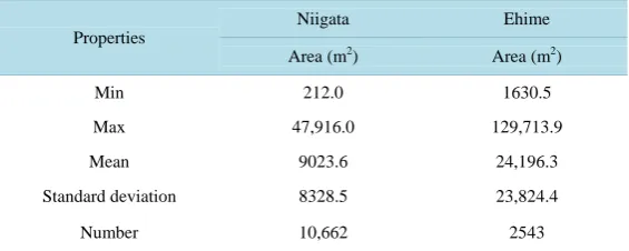
prepared by interpreting 1:40,000 aerial photographs. While the inventory includes many historical landslides identified from topographical discontinuities, small slope disturbances were not included. The use of historical (geomorphological) landslide inventories, which summarize past multiple landslide events [40], may enable a robust LSM because it reflects various environmental conditions, and the number of available data tends to be large. However, because of the uncertainties associated with the identification of large failures as unique (single) events [41], and lack of differentiation among landslide types (possible inclusion of slow moving earth flows), exceptionally large landslides greater than the 95th percentile of the land-slide area (Figure 3) were not used in this study. Table 1 shows the properties of the investigated landslides.

4. Methodology

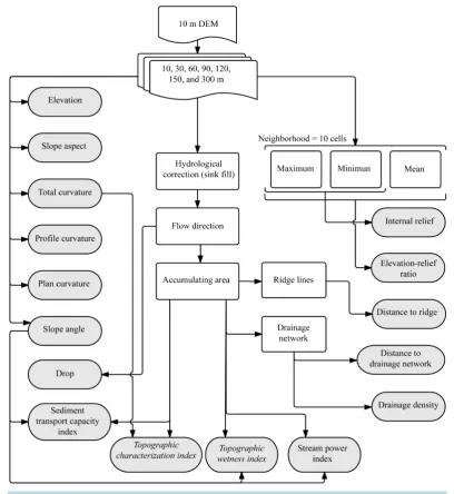
Topographic parameters were derived from the 10 m DEM. Random Forest was used to construct LS models using the topographic parameters and the landslide inventory. It was implemented in JMP Pro 11.2 (SAS Insti-tute Inc., Cary, NC), and GIS based calculations were performed using ArcGIS 10.3 (ESRI, Redlands, CA) and Python 2.7.

4.1. Topographic Parameters

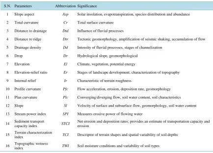
This study employs 16 DEM-derived topographic parameters (Figure 4, Table 2) previously used in landslide research [1][42]-[44]. Elevation (El) is a measure of the height of a surface above mean sea level. Slope (Sl) in-dicates the degree of inclination of the surface and shows the rate of elevation change. Slope aspect (Asp) represents the direction of the maximum slope. Drop (Dr), equivalent to the hydrologic slope [45][46], shows the ratio of the maximum change in elevation along the direction of flow between cell-centers. It provides an exact measure of surface inclination in relation to flow. Profile curvature (Pfc) is surface curvature in the direc-tion of slope and affects the acceleradirec-tion and deceleradirec-tion of surface flow. Plan curvature (Plc) is surface curva-ture perpendicular to slope direction and affects the convergence and divergence of surface flow. Total curvacurva-ture (Cr) reflects both the plan and profile curvatures and represents the overall surface curvature.

Ridges and channels are fundamental features of terrain morphology, and therefore are used in various terrain analyses [47]. In this study, drainage density (Dd), the total length per unit area, was computed using a circular

Figure 3. Percentile distribution of landslide area.

Table 1. Statistical properties of the studied landslides in Niigata and Ehime.

Properties

Niigata Ehime

Area (m2_{) Area (m}2₎

Min 212.0 1630.5

Max 47,916.0 129,713.9

Mean 9023.6 24,196.3

Standard deviation 8328.5 23,824.4

Figure 4. Interrelationship of the topographic parameters.

moving window of radius equaling the length of 10 cells. This unit area changing with DEM resolution allowed the mapping of drainage texture ranging from purely local to the regional average drainage density [48]. The shortest distance to a drainage line (Dtd) and shortest distance to a ridge (Dtr) were also computed. In areas of high seismicity, Dtr is a significant LS parameter reflecting the amplified motion observed at mountain tops [49]. Cells with flow accumulation higher than a threshold value were identified as drainage networks, while ridges were defined as lines of cells with zero flow accumulation.

Relative relief or internal relief (Ir) is the maximum elevation difference in a unit area [42]. The elevation- relief ratio (Er) describes the area distribution at different elevations and is defined as:

(

) (

)

Er= − − (1)

Table 2. Topographic parameters used for susceptibility modeling.

S.N. Parameters Abbreviation Significance

1 Slope aspect Asp Solar insolation, evapotranspiration, species distribution and abundance

2 Total curvature Cr Total surface curvature

3 Distance to drainage Dtd Influence of fluvial processes

4 Distance to ridge Dtr Tectonic geomorphology, amplification of seismic shaking, accumulation of flow

5 Drainage density Dd Intensity of fluvial processes, stages of channelization

6 Drop Dr Hydrological slope, geomorphological

7 Elevation El Climate, vegetation, potential energy

8 Elevation-relief ratio Er Stages of landscape development; characterization of topography

9 Internal relief Ir Characteristic of terrain roughness

10 Profile curvature Pfc Flow acceleration, erosion, deposition rate, geomorphology

11 Plan curvature Plc Converging/diverging flow, soil water content, soil characteristics

12 Slope Sl Velocity of surface and subsurface flow, geomorphology, soil water content

13 Stream power index SPI Measures erosive power of flowing water

14 Sediment transport

capacity index STCI

Net erosion and deposition rates; provides an estimate of transportation capacity and erosion

15 Terrain characterization

index TCI Descriptor of terrain shapes and spatial variability of soil depths

16 Topographic wetness

index TWI Soil moisture conditions and variability of soil types

features with the 10 m DEM and coarser-scale form of hillslope with the coarser DEMs) [54].

The sediment transport capacity index (STCI) is equivalent to the length-slope factor of the Revised Universal Soil Loss Equation [43]. Therefore, it accounts for the effects of topography on both sediment transport and ero-sion [55]. STCI is calculated as:

(

)(

) (

)

STCI= m+ A β (2)

where A is the upslope contributing area (m2), β is the local slope gradient (in degrees), and m and n are con-stants. Because the sensitivity of erosion predictions is not strongly affected by the values of the constants [56], the values m = 0.4 and n = 1.3 suggested by Chen and Yu [43] for Taiwan, an area of landslide activity compa-rable to our study areas, were used in this study.

The stream power index (SPI) also describes the potential of channel erosion and sediment transport processes

[55]. It is defined as:

(

)

ln tan

SPI= As× β (3)

where As is the specific catchment area (upslope contributing area per unit contour length).

TCI is related to the spatial variability of soil depth and sediment transportation capacity [26][57] and is de-fined as:

ln

TCI=Cr× As (4) TWI has been used to describe soil moisture distribution and has been found useful for landslide susceptibility studies; higher TWI values are often found in landslide bodies [21][43]. It is defined as:

(

)

ln tan

TWI= As β (5)

of other parameters according to the parameter ranking provided by the RF model [17].

Although the DEM-derived parameters represent distinct terrain properties and processes, their interrelation-ship may lead to multicollinearity. However, for LSM, Harrell [58] suggests that multicollinearity does not in-fluence the predictions from training and testing datasets if both have the same type of collinearities. This ap-plies to our study because all parameters used with the training and testing datasets are mathematical derivatives of the same 10 m DEM.

4.2. Random Forest

RF is an ensemble learning method of classification using regression trees which combines the idea of bagging with random feature selection [59]-[62]. RF utilizes bootstrap and random techniques to select the subsample of data and predictor parameters while growing an ensemble of trees (hence called “forest”). In addition to con-structing each tree using a different bootstrap sample of the data, RF changes how the classification or regres-sion trees are constructed. In classical deciregres-sion trees, each node is split using the best split among all parameters. In RF, by contrast, each node is split using the best among a subset of predictors randomly chosen at that node. This strategy leads to higher performance than many other classifiers such as discriminant analysis, SVM, and ANN; it also makes RF robust against overfitting [59][63]. RF has several other advantages: 1) it does not re-quire assumptions on the distribution of explanatory parameters; 2) it allows for the mixed use of categorical and numerical parameters without using dummy parameters; 3) it can account for interactions and nonlinearities between parameters [17].

RF produces multiple outputs to aid the interpretation of results, including out-of-bag (OOB) accuracy esti-mates and parameter importance measures [64]. OOB errors from RF classifications provide an alternative to cross-validation. For each tree in the forest, a random third of all observations are held out from the training set, and are referred to as OOB. The OOB error is, thus, the proportion of misclassified observations. The other cru-cial output is the measure of parameter importance, i.e., the statistical weight of each predictor variable. This study employs this measure to analyze the influence of scale on landslide causative parameters. OOB accuracy estimates provide the predictive efficacy of RF models. The change in generalized R-square (R2), a measure of variance in the dependent variable explained by the independent variables, was analyzed to identify the required number of trees.

Classification data used in an RF model for LSM should contain information about both landslides and no- landslide areas. A single-pixel sampling strategy using the centroid of a landslide polygon was employed. No- landslide points, whose number is equal to the number of landslides, were randomly created in no-landslide areas. Values of parameters for the landslide and no-landslide points were extracted. The data (50% landslide and 50% no-landslide) for Niigata and Ehime consist of 21,324 and 5086 entries, respectively. The data were randomly divided into training (50%) and testing (50%) datasets.

4.3. Multi-Resolution LSM

The seven DEM-scales (10 to 300 m) were applied to construct RF models classifying landslide presence and absence to identify the optimal resolution for each parameter. Figure 5(a) outlines the process. First, the values of the 16 parameters are computed for all the scales, and the values are used in an RF model to classify the landslide data. The scale of each parameter with the highest importance in the classification, determined as an average of 10 iterations, is considered optimal. This process is repeated for all the parameters, and finally, a combination of all parameters at their optimal scales is used to create a multi-resolution LS model and an LS map. The finest grid size among the parameters at their optimal scales is selected as the mapping unit. Figure 5(b) outlines the determination of parameter importance in a multi-resolution LS model. In the hypothetical example shown in Figure 5, Sl at 30 m contributes most to the classification, and therefore is the most important parameter for the LS study.

5. Results

Figure 5. Outline of multi-resolution technique for: (a) selection of optimal parameter scale and (b) determination of parameter importance.

Figure 6. Generalized R-squared and number of in an RF model.

Table 3and Table4 show the contribution of each parameter in the RF model at each scale for Niigata and Ehime, respectively. The results show that the optimal scale with the highest contribution differs among para-meters.

Table 3. Contribution of each parameter and each scale to modeling landslide distribution in Niigata. The highest contributor is selected as optimal (averaged over 10 iterations, RF T# 500).

Parameters Scales

Optimal 10 30 60 90 120 150 300

Asp 300 0.113 0.108 0.112 0.131 0.152 0.146 0.238

Cr 60 0.085 0.171 0.280 0.192 0.121 0.099 0.052

Dtd 10 0.347 0.226 0.126 0.093 0.075 0.072 0.061

Dtr 60 0.151 0.256 0.265 0.139 0.074 0.048 0.067

Dd 300 0.168 0.166 0.128 0.113 0.125 0.115 0.185

Dr 60 0.153 0.178 0.217 0.164 0.123 0.102 0.061

El 30 0.176 0.189 0.152 0.124 0.111 0.107 0.141

Er 10 0.198 0.170 0.116 0.144 0.114 0.117 0.140

Ir 10 0.356 0.211 0.112 0.071 0.057 0.080 0.112

Pfc 60 0.084 0.152 0.286 0.206 0.126 0.094 0.053

Plc 60 0.129 0.198 0.237 0.156 0.117 0.090 0.074

Sl 10 0.232 0.214 0.210 0.123 0.087 0.062 0.072

SPI 60 0.101 0.214 0.259 0.153 0.104 0.081 0.088

STCI 60 0.089 0.232 0.258 0.158 0.113 0.077 0.073

TCI 60 0.045 0.139 0.282 0.187 0.137 0.108 0.102

TWI 30 0.120 0.224 0.221 0.155 0.105 0.079 0.095

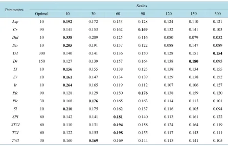
Table 4. Contribution of each parameter and each scale to modeling landslide distribution in Ehime. The highest contributor is selected as optimal (averaged over 10 iterations, RF T# 500).

Parameters Scales

Optimal 10 30 60 90 120 150 300

Asp 10 0.192 0.172 0.153 0.128 0.124 0.110 0.121

Cr 90 0.141 0.153 0.162 0.169 0.132 0.141 0.103

Dtd 10 0.338 0.209 0.125 0.116 0.080 0.079 0.052

Dtr 10 0.205 0.191 0.157 0.122 0.088 0.147 0.089

Dd 300 0.140 0.141 0.136 0.150 0.128 0.151 0.154

Dr 150 0.127 0.139 0.157 0.164 0.138 0.180 0.095

El 10 0.156 0.155 0.138 0.125 0.138 0.134 0.155

Er 10 0.161 0.147 0.134 0.139 0.129 0.138 0.152

Ir 10 0.264 0.165 0.119 0.112 0.107 0.106 0.127

Pfc 90 0.128 0.129 0.150 0.176 0.138 0.159 0.120

Plc 30 0.168 0.176 0.165 0.163 0.114 0.113 0.101

Sl 10 0.210 0.175 0.162 0.137 0.116 0.105 0.094

SPI 60 0.142 0.141 0.181 0.140 0.113 0.161 0.122

STCI 60 0.110 0.131 0.194 0.158 0.124 0.164 0.119

TCI 60 0.122 0.153 0.198 0.155 0.117 0.143 0.111

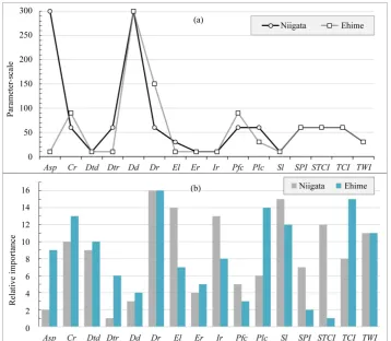
contribute the most at 300 m, the coarsest resolution. The results from Ehime are similar. For Ehime, parameters Asp, Dtd, Dtr, El, Er, Ir, and Sl are optimal at the finest scale, whereas the other parameters exhibit optima at coarser scales. Similar to Niigata, Dd in Ehime was found to be optimum at the coarsest scale. Figure 7(a)

compares the optimal parameter scale between the two study areas. The optimal scales for most parameters show similarity in both areas except Asp,for which the coarsest resolution in Niigata and the finest resolution in Ehime are optimal.

The relative importance of each optimal parameter is shown in Figure 7(b). Parameters Dr, Sl, El, Ir, STCI, and TWI for Niigata and Dr, TCI, Plc, Cr, Sl, and TWI for Ehime constitute the top six parameters explaining the distribution of landslides in each area. Parameters with higher relative importance (≥8; Figure 7(b)) in both areas are Cr, Dtd, Dr, Ir, Sl, TCI, and TWI. Some parameters were found to be of greater importance in one area but not in the other. The parameters with large differences in relative importance between the two areas (≥5;

Figure 7(b)) are Asp, El, Ir Plc, SPI, STCI, and TCI; Parameters El, Ir, SPI, and STCI have higher importance in Niigata while Asp, Plc, and TCI have higher importance in Ehime. The random variable “rand” was correctly identified as the least important parameter in the analysis.

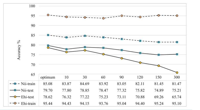
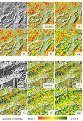
Figure 8 presents the testing and training accuracies of the RF models (averaged over 10 iterations) con-structed with parameters at various scales. In both areas, the training accuracies (85.08% for Niigata and 95.44% for Ehime) and testing accuracies (79.70% and 78.62%) were found to be highest for the models with parame-ters at the optimal scales. Among the model iterations, the models closest to the mean testing accuracy were used to produce LS maps. Figure 9 shows 25 km2 parts of the LS maps for the combined optimal scale and the 10, 30, 90, and 150 m scales.

The effectiveness of the model with parameters at the optimal scales was evaluated using receiver operating characteristics (ROC). The area under the ROC curve (AUC) characterizes the quality of a prediction model [65]. AUC values range from 0 to 1, and values closer to 1 represent a better classification model. Figure 10 illu-strates AUC values on test data for RF models at different scales. The model with the parameters at optimal

Figure 8. Training and testing accuracies of LS models for different parameter scales for Niigata and Ehime (averaged over 10 iterations, RF T# 500) (Nii-train = training samples at Niigata; Nii-test = testing samples at Niigata; Ehi-train = training samples at Ehime; and Ehi-test = training samples at Ehime).

scales shows an AUC value of 0.877 for Niigata and 0.870 for Ehime. The highest AUC values show that mul-ti-resolution LS modeling outperforms the conventional single scale modeling.

6. Discussion

Different terrain parameters vary in different ways when the DEM resolution changes [66]. This study has shown that the optimum scales for LS modeling also differ according to parameter (Table 3 and Table4), and they tend to be common for the two study areas (Figure 7(a)). Although it is expected that the finest DEM can describe detailed topography and is hence suitable for LSM, several parameters are more significant at relatively coarse scales (≥30 m). This suggests that the smallest-scale variabilities of these parameters do not well re- present the physical processes of landslide triggering, as suggested by some previous studies [25][67]. For ex-ample, all curvature-related variables (Cr, Pfc, and Plc) and the composite topographic indices (SPI, STCI, TCI, and TWI) show meaningful influences on landslide susceptibility at scales equal to or larger than 30 m (Figure 7(a)). This suggests that a 3 × 3 moving window for parameter computation properly encompasses a meaningful topographic unit, including both the detachment and deposition areas of a landslide, only at relatively coarse resolutions [17]. The landslide size distribution of the two study areas (Figure 3,Table 1) also suggests that most landslides are larger than the terrain represented at 10 m resolution. Scaling of Dr with the optimal 60 or 150 m resolution also seems to correspond to the landslide size distribution. In contrast, for Ir and Er, the finest resolution (10 m) is the optimal scale for both areas, and it is ascribable to a larger 10 × 10 moving window used for their computation, which can represent a relatively large area even at the finest resolution. However, al-though computed using a 3 × 3 moving window, Sl is optimal at the finest scale. This seems to reflect the high sensitivity of slope calculation to DEM resolution. It is widely known that lower resolution DEMs result in low-er Sl values for the same terrain [68]. Because Sl is directly related to gravitational force triggering landslides, its accurate computation using fine DEMs is important. A similar explanation can be given for Dtd, which is also optimal at the finest 10 m scale. Fluvial activity such as channel erosion tends to induce landslides along the river course. The accurate location of rivers is better represented if the finest DEM is used [69].

Figure 9. Landslide distribution map (grey) and part of LS maps (25 km2 and probability ≥ 0.5)

from RF models with different parameter scales for Niigata (upper) and Ehime (lower).

Figure 10. AUC values of ROC curves for test data for the models at various scales (left). ROC

were due to high seismicity, as was the case of the 2004 Chuestu earthquake [71].

The optimal scales of Dd and Asp differ significantly from those of the other parameters; the coarsest scale (300 m) is optimum for Dd, while Asp shows the largest deviation between the two areas, 10 and 300 m. Dd in this study is estimated over a unit area dependent on the scale of analysis, thus at finer scales itmight be related only to the local presence/absence of drainage lines. However, at coarser scales, it can reflect the known rela-tionship between general relief characteristics and landslide occurrences [51][72][73]. For Asp, the finest reso-lution (10 m) is optimal for Ehime, while the coarsest resoreso-lution (300 m) is optimal for Niigata. Local meteoro-logical conditions and their relationship with LS may explain this variation. Both the study areas receive large amounts of precipitation; however, Niigata receives a significant portion of its precipitation as snowfall (1.35 m per year). The increased overburden due to accumulated snow and the increased soil moisture from snowmelt are responsible for landslides there [74]. Asp at a coarser scale indicates the overall direction of a hillslope and suggests that the difference in the deposition thickness of snow on the windward and leeward sides is crucial for LS in Niigata. In contrast, Asp at a finer scale could depict local variations in micro-climate, such as insolation and related groundwater conditions, which is related to rock weathering [75]. The close relationship between weathering and distribution of landslides has been reported in Shikoku Island including Ehime [76], indicating the effect of finer scale Asp on local climate, weathering, and landslides.

6.2. Parameter Importance

Among the values of relative parameter importance (Figure 7(b)), higher values for Cr, Dtd, Dr, Ir, Sl, TCI, and TWI in both study areas suggest that these parameters are instrumental in landslide occurrences. Landslide probability generally increases with terrain slope because of increased shear stress, and slope is considered very important in LS studies [77][78]. Therefore, the higher importance of Dr and Sl is reasonable. The higher im-portance of Dr compared to Sl confirms that Dr is a more direct representation of local maximum slope. Claessens et al. [45] provided a similar observation on the different effects of these slope parameters. The higher importance of Ir in both study areas also suggests the importance of topographic steepness.

The importance of Dtd is explained by the bidirectional relationship between fluvial processes and slope fail-ures. While landslides contribute to channel initiation, stream incision also contributes to landslides [73] [79]-[81]. The higher relative importance of TCI and TWI may reflect the significance of hydrological variations related to rock weathering and soil properties [21] [82] [83]. There is a general consensus regarding Cr that landslides are more likely to occur on concave slopes because of groundwater concentration [84]. In contrast, earthquake-induced landslides may be more likely on convex slopes with higher ground acceleration. The im-portance of Cr in both study areas therefore hints to such mechanisms controlling LS.

Parameters Asp, Plc, and TCI have markedly higher importance in Ehime than in Niigata. A combination of geological and environmental variables may explain this observation. As noted, the importance of Asp in Ehime may be due to local micro-climatic differences that lead to differential weathering. By contrast, the higher im-portance of Plc in Ehime indicates the positive influence of horizontal flow movement in LS, as suggested by Nefeslioglu et al. [77] (Table 2). The area in Ehime receives a larger amount of rainfall than in Niigata, hence increased water concentration may contribute more to landslides. The higher importance of TCI in Ehime can be explained similarly because it is a parameter strongly related to terrain curvature.

For Niigata, the relative importance of El, Ir, SPI,and STCI are evidently higher than in Ehime. The effects of El and Ir may be related to the effects of earthquakes because higher or high-relief areas tend to undergo accele-rated seismic movement. SPI and STCI provide measures of erosion by water flowing from the entire upstream area (Table 2). They are hydrological parameters but are different from curvatures that reflect much more loca-lized water concentration and divergence. The importance of curvature in Ehime and that of SPI and STCI in Niigata suggest that hilly and gentler terrain in Niigata requires not local but wider-scale water concentration for active landslides.

6.3. Assessment of LS Models

scale beyond 30 m. The slight increase in the model accuracy for Niigata at 300 m is the effect of the two para-meters that are optimal at that scale (Figure 7(a)). The discrepancy observed with the training accuracies for Ehime might be due to the smaller number of training samples. Higher testing accuracies were obtained for models at coarser scales (≥30 m) than at the finest scale (10 m). The proposed multi-resolution LS technique re-sulted in a boost of testing accuracies according to the obtained AUC values (Figure 10).

Figure 9 shows examples of local LS maps at different scales. The figure indicates that the usability of an LS map depends on the mapping scale as well as the model used. Selection of mapping scale of each parameter for the proposed multi-resolution approach enables us to achieve higher accuracy LSM.

7. Conclusions

LSM provides the relative likelihood of future landslides, conditional on local geomorphic and topographic cha-racteristics [85]. Results of our LS study suggest that a single parameter-scale analysis falls short in accommo-dating the heterogeneity of geomorphological characteristics of the landslides and their surrounding area. This study proposes a multi-resolution LSM technique to incorporate such variabilities. The method requires an iden-tification of optimum scales for all parameters to best represent the conditions of slope failure. The parameters at different optimum scales are then brought together for the final LSM.

The study has also demonstrated the usefulness of a DEM-based LS analysis in areas without other sets of high-quality thematic data. The analysis of scale and importance of the DEM-derived parameters reveal that while some parameters show similar importance and scale dependency for different regions, environmental dif-ferences result in variability between regions. The performance of LS models also suggests that the finest scale of analysis is not always the best. The proposed multi-resolution LS analysis permits higher accuracy LSM than any single-scale analysis. Further study of different areas is necessary to confirm the usefulness of the multi- resolution approach.

References

[1] Guzzetti, F., Carrara, A., Cardinali, M. and Reichenbach, P. (1999) Landslide Hazard Evaluation: A Review of Current Techniques and Their Application in a Multi-Scale Study, Central Italy. Geomorphology, 31, 181-216.

http://dx.doi.org/10.1016/S0169-555X(99)00078-1

[2] Brabb, E. (1984) Innovative Approaches to Landslide Hazard Mapping. 4th International Symposium on Landslides. Toronto, 307-324.

[3] Varnes, D.J. (1984) Landslide Hazard Zonation: A Review of Principles and Practice, Natural Hazards. UNESCO, Paris.

[4] Hussin, H.Y., Zumpano, V., Reichenbach, P., Sterlacchini, S., Micu, M., van Westen, C. and Bălteanu, D. (2015) Dif-ferent Landslide Sampling Strategies in a Grid-Based Bi-Variate Statistical Susceptibility Model. Geomorphology, 253, 508-523. http://dx.doi.org/10.1016/j.geomorph.2015.10.030

[5] Atkinson, P.M. and Massari, R. (1998) Mapping Susceptibility to Landsliding in the Central Apennines, Italy. Com-puters and Geosciences, 24, 373-385. http://dx.doi.org/10.1016/S0098-3004(97)00117-9

[6] Yalcin, A., Reis, S., Aydinoglu, A.C. and Yomralioglu, T. (2011) A GIS-Based Comparative Study of Frequency Ratio, Analytical Hierarchy Process, Bivariate Statistics and Logistics Regression Methods for Landslide Susceptibility Map-ping in Trabzon, NE Turkey. Catena, 85, 274-287. http://dx.doi.org/10.1016/j.catena.2011.01.014

[7] Ayalew, L. and Yamagishi, H. (2005) The Application of GIS-Based Logistic Regression for Landslide Susceptibility Mapping in the Kakuda-Yahiko Mountains, Central Japan. Geomorphology, 65, 15-31.

http://dx.doi.org/10.1016/j.geomorph.2004.06.010

[8] Akgun, A. (2011) A Comparison of Landslide Susceptibility Maps Produced by Logistic Regression, Multi-Criteria Decision, and Likelihood Ratio Methods: A Case Study at İzmir, Turkey. Landslides, 9, 93-106.

http://dx.doi.org/10.1007/s10346-011-0283-7

[9] Regmi, N.R., Giardino, J.R. and Vitek, J.D. (2010) Modeling Susceptibility to Landslides Using the Weight of Evi-dence Approach: Western Colorado, USA. Geomorphology, 115, 172-187.

http://dx.doi.org/10.1016/j.geomorph.2009.10.002

[10] Conforti, M., Pascale, S., Robustelli, G. and Sdao, F. (2014) Evaluation of Prediction Capability of the Artificial Neur-al Networks for Mapping Landslide Susceptibility in the Turbolo River Catchment (Northern CNeur-alabria, ItNeur-aly). Catena, 113, 236-250. http://dx.doi.org/10.1016/j.catena.2013.08.006

Support Vector Machines, Decision Tree, and Nave Bayes Models. Mathematical Problems in Engineering, 2012, 1-

26. http://dx.doi.org/10.1155/2012/974638

[12] Saito, H., Nakayama, D. and Matsuyama, H. (2009) Comparison of Landslide Susceptibility Based on a Decision-Tree Model and Actual Landslide Occurrence: The Akaishi Mountains, Japan. Geomorphology, 109, 108-121.

http://dx.doi.org/10.1016/j.geomorph.2009.02.026

[13] Díaz-Uriarte, R. and Alvarez de Andrés, S. (2006) Gene Selection and Classification of Microarray Data Using Ran-dom Forest. BMC Bioinformatics, 7, 3. http://dx.doi.org/10.1186/1471-2105-7-3

[14] Lin, W.-Z., Fang, J.-A., Xiao, X. and Chou, K.-C. (2011) iDNA-Prot: Identification of DNA Binding Proteins Using Random Forest with Grey Model. PLoS One, 6, e24756. http://dx.doi.org/10.1371/journal.pone.0024756

[15] Cutler, D.R., Edwards, T.C., Beard, K.H., Cutler, A., Hess, K.T., Gibson, J. and Lawler, J.J. (2007) Random Forest for Classification in Ecology. Ecology, 88, 2783-2792. http://dx.doi.org/10.1890/07-0539.1

[16] Brenning, A. (2005) Spatial Prediction Models for Landslide Hazards: Review, Comparison and Evaluation. Natural Hazards and Earth System Sciences, 5, 853-862. http://dx.doi.org/10.5194/nhess-5-853-2005

[17] Catani, F., Lagomarsino, D., Segoni, S. and Tofani, V. (2013) Landslide Susceptibility Estimation by Random Forests Technique: Sensitivity and Scaling Issues. Natural Hazards and Earth System Sciences, 13, 2815-2831.

http://dx.doi.org/10.5194/nhess-13-2815-2013

[18] Vorpahl, P., Elsenbeer, H., Märker, M. and Schröder, B. (2012) How Can Statistical Models Help to Determine Driv-ing Factors of Landslides? Ecological Modelling, 239, 27-39. http://dx.doi.org/10.1016/j.ecolmodel.2011.12.007

[19] Hasegawa, S., Dahal, R.K., Nishimura, T., Nonomura, A. and Yamanaka, M. (2009) DEM-Based Analysis of Earth-quake-Induced Shallow Landslide Susceptibility. Geotechnical and Geological Engineering, 27, 419-430.

http://dx.doi.org/10.1007/s10706-008-9242-z

[20] Coblentz, D., Pabian, F. and Prasad, L. (2014) Quantitative Geomorphometrics for Terrain Characterization. Interna-tional Journal of Geosciences, 5, 247-266. http://dx.doi.org/10.4236/ijg.2014.53026

[21] Moore, I., Gessler, P., Nielsen, G.A. and Peterson, G.A. (1993) Soil Attribute Prediction Using Terrain Analysis. Soil Science Society of America Journal, 57, 443-452. http://dx.doi.org/10.2136/sssaj1993.03615995005700020026x

[22] Prima, O.D.A. and Yoshida, T. (2010) Characterization of Volcanic Geomorphology and Geology by Slope and Topo-graphic Openness. Geomorphology, 118, 22-32. http://dx.doi.org/10.1016/j.geomorph.2009.12.005

[23] Crozier, M.J. and Glade, T. (2012) A Review of Scale Dependency in Landslide Hazard and Risk Analysis. In:Glade, T., Anderson, M. and Crozier, M.J., Eds., Landslide Hazard and Risk, John Wiley & Sons, Ltd.,Chichester, 75-138. [24] Keijsers, J.G.S., Schoorl, J.M., Chang, K.T., Chiang, S.H., Claessens, L. and Veldkamp, A. (2011) Calibration and

Resolution Effects on Model Performance for Predicting Shallow Landslide Locations in Taiwan. Geomorphology, 133, 168-177. http://dx.doi.org/10.1016/j.geomorph.2011.03.020

[25] Tarolli, P. and Tarboton, D.G. (2006) A New Method for Determination of Most Likely Landslide Initiation Points and the Evaluation of Digital Terrain Model Scale in Terrain Stability Mapping. Hydrology and Earth System Sciences, 10, 663-677. http://dx.doi.org/10.5194/hess-10-663-2006

[26] Catani, F., Segoni, S. and Falorni, G. (2010) An Empirical Geomorphology-Based Approach to the Spatial Prediction of Soil Thickness at Catchment Scale. Water Resources Research, 46, W05508.

http://dx.doi.org/10.1029/2008wr007450

[27] Yamagishi, H., Ayalew, L., Horimatsu, T., Kanno, T. and Hatamoto, M. (2004) Recent Landslides in Niigata Region, Japan [WWW Document]. Japan Landslide Soc.

http://www.landslide-soc.org/e-content/Recent_landslides_in_Niigata_region.pdf

[28] Yoshimatsu, H. and Abe, S. (2006) A Review of Landslide Hazards in Japan and Assessment of Their Susceptibility Using an Analytical Hierarchic Process (AHP) Method. Landslides, 3, 149-158.

http://dx.doi.org/10.1007/s10346-005-0031-y

[29] Geological Survey of Japan (1995) Strip Map of the Itoigawa-Shizuoka Tectonic Line Active Fault System, 1:100,000. (In Japanese with English Abstract)

[30] Inoue, K., Mori, T. and Mizuyama, T. (2012) Three Large Historical Landslide Dams and Outburst Disasters in the North Fossa Magna Area, Central Japan. International Journal of Electrical and Computer Engineering (IJECE), 5, 145-154. http://dx.doi.org/10.13101/ijece.5.134

[31] Takeda, T., Sato, H., Iwasaki, T., Matsuta, N., Sakai, S., Iidaka, T. and Kato, A. (2004) Crustal Structure in the North-ern Fossa Magna Region, Central Japan, Modeled from Refraction/Wide-Angle Reflection Data. Earth, Planets and Space, 56, 1293-1299.

[33] Has, B., Noro, T., Maruyama, K., Nakamura, A., Ogawa, K. and Onoda, S. (2012) Characteristics of Earthquake-In- duced Landslides in a Heavy Snowfall Region-Landslides Triggered by the Northern Nagano Prefecture Earthquake, March 12, 2011, Japan. Landslides, 9, 539-546. http://dx.doi.org/10.1007/s10346-012-0344-6

[34] Matsuda, T., Nakamura, K. and Sugimura, A. (1967) Late Cenozoic Orogeny in Japan. Tectonophysics, 4, 349-366.

http://dx.doi.org/10.1016/0040-1951(67)90004-2

[35] Takeuchi, A. (2004) Basement-Involved Tectonics in North Fossa Magna, Central Japan: The Significance of the Northern Itoigawa-Shizuoka Tectonic Line. Earth, Planets and Space, 56, 1261-1269.

http://dx.doi.org/10.1186/BF03353349

[36] Nakazato, H., Shoda, D., Inoue, K. and Suzuki, H. (2013) A Case Study of Behavior Observation of Landslide Induced by Snowmelt After an Earthquake. In: Ugai, K., Yagi, H. and Wakai, A., Eds., Earthquake-Induced Landslides: Pro-ceedings of the International Symposium on Earthquake-Induced Landslides, Kiryu, Japan, 2012, Springer, Berlin, 341-345. http://dx.doi.org/10.1007/978-3-642-32238-9_35

[37] Banno, S. and Sakai, C. (1989) Geology and Metamorphic Evolution of the Sanbagawa Metamorphic Belt, Japan.

Geological Society of London, Special Publication, 43, 519-532. http://dx.doi.org/10.1144/GSL.SP.1989.043.01.50

[38] Suzuki, S. and Ishizuka, H. (1998) Low-Grade Metamorphism of the Mikabu and Northern Chichibu Belts in Central Shikoku, SW Japan: Implications for the Areal Extent of the Sanbagawa Low-Grade Metamorphism. Journal of Me-tamorphic Geology, 16, 107-116. http://dx.doi.org/10.1111/j.1525-1314.1998.00066.x

[39] Hong, Y., Hiura, H., Shino, K., Sassa, K., Suemine, A., Fukuoka, H. and Wang, G. (2005) The Influence of Intense Rainfall on the Activity of Large-Scale Crystalline Schist Landslides in Shikoku Island, Japan. Landslides, 2, 97-105.

http://dx.doi.org/10.1007/s10346-004-0043-z

[40] Malamud, B.D., Turcotte, D.L., Guzzetti, F. and Reichenbach, P. (2004) Landslide Inventories and Their Statistical Properties. Earth Surface Processes and Landforms, 29, 687-711. http://dx.doi.org/10.1002/esp.1064

[41] Guzzetti, F., Malamud, B.D., Turcotte, D.L. and Reichenbach, P. (2002) Power-Law Correlations of Landslide Areas in Central Italy. Earth and Planetary Science Letters, 195, 169-183. http://dx.doi.org/10.1016/S0012-821X(01)00589-1

[42] Castellanos Abella, E.A. and Van Westen, C.J. (2008) Qualitative Landslide Susceptibility Assessment by Multicriteria Analysis: A Case Study from San Antonio del Sur, Guantánamo, Cuba. Geomorphology, 94, 453-466.

http://dx.doi.org/10.1016/j.geomorph.2006.10.038

[43] Chen, C.-Y. and Yu, F.-C. (2011) Morphometric Analysis of Debris Flows and Their Source Areas Using GIS. Geo-morphology, 129, 387-397. http://dx.doi.org/10.1016/j.geomorph.2011.03.002

[44] Nefeslioglu, H.A., Duman, T.Y. and Durmaz, S. (2008) Landslide Susceptibility Mapping for a Part of Tectonic Kelkit Valley (Eastern Black Sea Region of Turkey). Geomorphology, 94, 401-418.

http://dx.doi.org/10.1016/j.geomorph.2006.10.036

[45] Claessens, L., Heuvelink, G.B.M., Schoorl, J.M. and Veldkamp, A. (2005) DEM Resolution Effects on Shallow Landslide Hazard and Soil Redistribution Modelling. Earth Surface Processes and Landforms, 30, 461-477.

http://dx.doi.org/10.1002/esp.1155

[46] Tarboton, D.G. (1997) A New Method for the Determination of Flow Directions and Upslope Areas in Grid Digital Elevation Models. Water Resources Research, 33, 309-319. http://dx.doi.org/10.1029/96WR03137

[47] Band, L.E. (1986) Topographic Partition of Watersheds with Digital Elevation Models. Water Resources Research, 22, 15-24. http://dx.doi.org/10.1029/WR022i001p00015

[48] Tucker, G.E., Catani, F., Rinaldo, A. and Bras, R.L. (2001) Statistical Analysis of Drainage Density from Digital Ter-rain Data. Geomorphology, 36, 187-202. http://dx.doi.org/10.1016/S0169-555X(00)00056-8

[49] Chang, K.-T., Chiang, S.-H. and Hsu, M.-L. (2007) Modeling Typhoon- and Earthquake-Induced Landslides in a Mountainous Watershed Using Logistic Regression. Geomorphology, 89, 335-347.

http://dx.doi.org/10.1016/j.geomorph.2006.12.011

[50] Pike, R.J. and Wilson, S.E. (1971) Elevation-Relief Ratio, Hypsometric Integral, and Geomorphic Area-Altitude Anal-ysis. Geological Society of America Bulletin, 82, 1079-1084.

http://dx.doi.org/10.1130/0016-7606(1971)82[1079:ERHIAG]2.0.CO;2

[51] Strahler, A.N. (1952) Hypsometric (Area-Altitude) Analysis of Erosional Topography. Geological Society of America Bulletin, 63, 1117-1142. http://dx.doi.org/10.1130/0016-7606(1952)63[1117:haaoet]2.0.co;2

[52] Pérez-Peña, J.V., Azañón, J.M., Booth-Rea, G., Azor, A. and Delgado, J. (2009) Differentiating Geology and Tectonics Using a Spatial Autocorrelation Technique for the Hypsometric Integral. Journal of Geophysical Research, 114, F02018.

[54] Staley, D.M. and Waskelwicz, T.A. (2013) The Use of Airborne Laser Swath Mapping on Fans and Cones: An Exam-ple from the Colorado Front Range. In: Schneuwly-Bollschweiler, M., Stoffel, M. and Rudolf-Miklau, F., Eds., Dating Torrential Processes on Fans and Cones, Springer, Dordrecht, 147-164.

http://dx.doi.org/10.1007/978-94-007-4336-6_9

[55] Moore, I.D., Grayson, R.B. and Ladson, A.R. (1991) Digital Terrain Modelling: A Review of Hydrological, Geomor-phological, and Biological Applications. Hydrological Processes, 5, 3-30. http://dx.doi.org/10.1002/hyp.3360050103

[56] Kitahara, H., Okura, Y., Sammori, T. and Kawanami, A. (2000) Application of Universal Soil Loss Equation (USLE) to Mountainous Forests in Japan. Journal of Forest Research, 5, 231-236. http://dx.doi.org/10.1007/BF02767115

[57] Park, S., McSweeney, K. and Lowery, B. (2001) Identification of the Spatial Distribution of Soils Using a Process- Based Terrain Characterization. Geoderma, 103, 249-272. http://dx.doi.org/10.1016/S0016-7061(01)00042-8

[58] Harrell Jr., F.E. (2001) Multivariable Modeling Strategies. In: Harrell Jr., F.E., Ed., Regression Modeling Strategies, Springer, New York, 53-85. http://dx.doi.org/10.1007/978-1-4757-3462-1_4

[59] Breiman, L. (2001) Random Forests. Machine Learning, 45, 5-32. http://dx.doi.org/10.1023/A:1010933404324

[60] Cutler, A., Cutler, D.R. and Stevens, J.R. (2012) Random Forests. In: Zhang, C. and Ma, Y.Q., Eds., Ensemble Ma-chine Learning, Springer, New York, 157-175. http://dx.doi.org/10.1007/978-1-4419-9326-7_5

[61] Breiman, L. (1996) Bagging Predictors. Machine Learning, 24, 123-140. http://dx.doi.org/10.1007/BF00058655

[62] Ho, T.K. (1998) The Random Subspace Method for Constructing Decision Forests. IEEE Transactions on Pattern Analysis and Machine Intelligence, 20, 832-844. http://dx.doi.org/10.1109/34.709601

[63] Liaw, A. and Wiener, M. (2002) Classification and Regression by Random Forest. R News, 2, 18-22.

[64] Bricher, P.K., Lucieer, A., Shaw, J., Terauds, A. and Bergstrom, D.M. (2013) Mapping Sub-Antarctic Cushion Plants Using Random Forests to Combine Very High Resolution Satellite Imagery and Terrain Modelling. PLoS ONE, 8, e72093. http://dx.doi.org/10.1371/journal.pone.0072093

[65] Yesilnacar, E. and Topal, T. (2005) Landslide Susceptibility Mapping: A Comparison of Logistic Regression and Neural Networks Methods in a Medium Scale Study, Hendek Region (Turkey). Engineering Geology, 79, 251-266.

http://dx.doi.org/10.1016/j.enggeo.2005.02.002

[66] Zhou, Q. and Chen, Y. (2011) Generalization of DEM for Terrain Analysis Using a Compound Method. ISPRS Journal of Photogrammetry and Remote Sensing, 66, 38-45. http://dx.doi.org/10.1016/j.isprsjprs.2010.08.005

[67] Freer, J., McDonnell, J.J., Beven, K.J., Peters, N.E., Burns, D.A., Hooper, R.P., Aulenbach, B. and Kendall, C. (2002) The Role of Bedrock Topography on Subsurface Storm Flow. Water Resources Research, 38, 1269.

http://dx.doi.org/10.1029/2001WR000872

[68] Zhang, X., Drake, N.A., Wainwright, J. and Mulligan, M. (1999) Comparison of Slope Estimates from Low Resolution DEMs: Scaling Issues and a Fractal Method for Their Solution. Earth Surface Processes and Landforms, 24, 763-779.

http://dx.doi.org/10.1002/(SICI)1096-9837(199908)24:9<763::AID-ESP9>3.0.CO;2-J

[69] Wang, X. and Yin, Z.Y. (1998) A Comparison of Drainage Networks Derived from Digital Elevation Models at Two Scales. Journal of Hydrology, 210, 221-241. http://dx.doi.org/10.1016/S0022-1694(98)00189-9

[70] ESRI (2016) Flow Accumulation (Spatial Analyst) [WWW Document]. ArcGIS Resour. Cent.

http://help.arcgis.com/En/Arcgisdesktop/10.0/Help/index.html#//009z00000051000000.htm

[71] Wang, H.B., Sassa, K. and Xu, W.Y. (2007) Analysis of a Spatial Distribution of Landslides Triggered by the 2004 Chuetsu Earthquakes of Niigata Prefecture, Japan. Natural Hazards, 41, 43-60.

http://dx.doi.org/10.1007/s11069-006-9009-x

[72] Lin, Z. and Oguchi, T. (2004) Drainage Density, Slope Angle, and Relative Basin Position in Japanese Bare Lands from High-Resolution DEMs. Geomorphology, 63, 159-173. http://dx.doi.org/10.1016/j.geomorph.2004.03.012

[73] Oguchi, T. (1997) Drainage Density and Relative Relief in Humid Steep Mountains with Frequent Slope Failure. Earth Surface Processes and Landforms, 22, 107-120.

http://dx.doi.org/10.1002/(SICI)1096-9837(199702)22:2<107::AID-ESP680>3.0.CO;2-U

[74] Kawagoe, S., Kazama, S. and Ranjan Sarukkalige, P. (2009) Assessment of Snowmelt Triggered Landslide Hazard and Risk in Japan. Cold Regions Science and Technology, 58, 120-129. http://dx.doi.org/10.1016/j.coldregions.2009.05.004

[75] Rech, J.A., Reeves, R.W. and Hendricks, D.M. (2001) The Influence of Slope Aspect on Soil Weathering Processes in the Springerville Volcanic Field, Arizona. Catena, 43, 49-62. http://dx.doi.org/10.1016/S0341-8162(00)00118-1

[76] Yamasaki, S. and Chigira, M. (2008) Weathering Mechanism of Pelitic Schist and Its Relationships with Landslides: Analysis of Undisturbed Drilled Cores from the Sambagawa Metamorphic Belt in Shikoku. Journal of the Geological Society of Japan, 114, 109-126. http://dx.doi.org/10.5575/geosoc.114.109

Geol-ogy, 47, 982-990. http://dx.doi.org/10.1007/s00254-005-1228-z

[78] Nefeslioglu, H.A., Gokceoglu, C. and Sonmez, H. (2008) An Assessment on the Use of Logistic Regression and Ar-tificial Neural Networks with Different Sampling Strategies for the Preparation of Landslide Susceptibility Maps. En-gineering Geology, 97, 171-191. http://dx.doi.org/10.1016/j.enggeo.2008.01.004

[79] Gerrad, A.J. and Gardner, R.A.M. (2000) The Role of Landsliding in Shaping the Landscape of the Middle Hills, Nep-al. Zeitschrift fur Geomorphologie Supplement, 122, 47-62.

[80] Montgomery, D.R. and Dietrich, W.E. (1989) Source Areas, Drainage Density, and Channel Initiation. Water Re-sources Research, 25, 1907-1918. http://dx.doi.org/10.1029/WR025i008p01907

[81] Ng, K.Y. (2006) Landslide Locations and Drainage Network Development: A Case Study of Hong Kong. Geomor-phology, 76, 229-239. http://dx.doi.org/10.1016/j.geomorph.2005.10.008

[82] Iwahashi, J. and Pike, R.J. (2007) Automated Classifications of Topography from DEMs by an Unsupervised Nested- Means Algorithm and a Three-Part Geometric Signature. Geomorphology, 86, 409-440.

http://dx.doi.org/10.1016/j.geomorph.2006.09.012

[83] Prima, O.D.A., Echigo, A., Yokoyama, R. and Yoshida, T. (2006) Supervised Landform Classification of Northeast Honshu from DEM-Derived Thematic Maps. Geomorphology, 78, 373-386.

http://dx.doi.org/10.1016/j.geomorph.2006.02.005

[84] Ayalew, L., Yamagishi, H. and Ugawa, N. (2004) Landslide Susceptibility Mapping Using GIS-Based Weighted Li-near Combination, the Case in Tsugawa Area of Agano River, Niigata Prefecture, Japan. Landslides, 1, 73-81.

http://dx.doi.org/10.1007/s10346-003-0006-9