MEASURING PROCESS INNOVATION ON DOUBLE FLANKED CONCEPTUAL MODEL FOR KNOWLEDGE SHARING ON ONLINE LEARNING ENVIRONMENT

(1)

1389

FINITE-DIFFERENTIAL SCHEME OF IDENTIFICATION OF

OVERALL HEAT EXCHANGE COEFFICIENT

1

A.BAIMANKULOV, 2A. ISMAILOV, 3T. ZHUASPAYEV

1

Professor, A. Baitursynov Kostanay StateUniversity, Kostanay, KAZAKHSTAN

2

Associate professor, A. Baitursynov Kostanay StateUniversity, Kostanay, KAZAKHSTAN

3

Senior lecturer, A. Baitursynov Kostanay StateUniversity, Kostanay, KAZAKHSTAN

E-mail: [email protected], [email protected], [email protected]

ABSTRACT

This work studies one-dimensional problem of heat distribution in matter. The measured value of soil temperature and near ground air temperature are set. Iteration method is proposed for defining overall heat exchange coefficient of multilayer material. The method is realized with the aid of finite-differential scheme, which gives solution, converging to the solution of differential problem. The result of numerical solutions of test problems are given.

Keywords: Heat Emission Coefficient, Finite-Differential Scheme, Iteration, Primal And Conjugate Problems, Functional, Initial Boundary Conditions

1. INTRODUCTION

In modern conditions, any solution of the economic nature in field of planning and prognosis of events on agricultural fields are based on the parameters of root zone and near-soil air layer. These parameters are to be measured extremely precise and used skillfully. Since all the possible agro-technical practices are conducted on fields, square of which are up to several hundreds of hectares, thus the information of the measurements should characterize mid-value of parameters for the whole square. Herewith, ground-based parameter measuring principle, presupposing their fixation in a single point of the field, is widely used. Numerous experiments, conducted by different scientists confirm a major dispersion of the results obtained. This is generally applied to the temperature of soil surface and deep profile, thermal characteristics and soil moisture level, and its density.

It is possible to obtain mid-value data for the whole field by means of elevating corresponding set of equipment to a certain level over the soil surface.

When problems of planning and regulating technological processes on agricultural fields are being solved, agricultural fields are understood as the soil and the air near it. Thus, it is necessary to know on what laws soil characteristics are based, not all the layers of it, but only the upper ones, i.e.

zones including ploughed layer, in which root systems are found, in which the regimes of heat, moisture, mechanical composition and density have direct influence on growth and development of seeds. The very soil layer, being dynamic in agro-biological sense, is called the active layer.

The study of laws of managing the features of soil active layer in many ways solve the problems of planning and regulating technological processes in the complex of “near ground air-soil”. Nowadays many methods of separate and complex definition of thermo-physical characteristics of materials are used. All those methods are widely used in engineering, scientific researches. Definition of thermo-physical characteristics demands the knowledge of head distribution in body or specimen, i.e. solution of initial boundary value problem of heat conductivity equation.

Some soil characteristics, i.e. parameters of functions were empirically composed in form of finite formula [1, 2, 3].

Influence of mass exchange on the coefficient of soil heat conductivity is experimentally studied by scientists [4, 5, 6, 7, 8].

Drawback of above mentioned methods is a definition of soil characteristics only for separately studied soil strips, which is a restriction for its wide application.

(2)

ISSN: 1992-8645 www.jatit.org E-ISSN: 1817-3195

1390 non-stationary methods, based of theory of solving thermal conductivity equation with non-stationary heat flow are stated in works [9, 10, 11, 12] and others.

The above mentioned methods are purposed for solving so-called linear initial boundary problem of heat conductivity equation for regular shapes (sphere, cylinder, parallelepiped and others) and with certain simplifications for input parameters.

Nowadays, the potential of mathematical modeling on one hand, allows to conduct a proper study of vital problems of the branch mentioned, on the other hand, newly emerging problems of theory and practice stimulate development of new methods and approaches of studying corresponding mathematics branches.

Computer modeling of heat and mass transfer allow to avoid the need of highly expensive natural experiments and to obtain solutions that are very close to reality.

Many practical problems demand the definition of initial heat distribution of the area, such problems are called initial boundary problems for equation of heat conductivity with reverse time.

Classification of reverse problems for parabolic equation is given in works [13, 14, 15] and others.

There works contain methods of numerical calculation based on proximal computational models and obtained results are compared to the experimental data.

Development and grounding of mathematical models of physical processes is solidly linked to solving reverse problems for differential equation.

Equation, describing the process of changing thermo-physical parameters, for which the reverse problem is set, is a mathematical model of a real soil mass. The model corresponding to a given information about the real state of active soil layer should be chosen from a given set of mathematical models. Reverse problems of mathematical physics are frequently set in a wrong way. This peculiarity of reverse problems is related to the basic difficulties of building efficient calculation algorithms.

Definition of correct input values for solving reverse coefficient problems in most cases were of a theoretical nature, or difficult to realize in practice. Which is why development of new methods of solving reverse problem of non-linear differential equations is always a difficult problem

In practical calculations, formulas obtained from differential problems are used. It is empirically proven that these computational models in most cases give major inaccuracy. This is why it is planned to develop new iteration methods, based on

discrete model of heat and mass exchange processes of soil within the project.

2. STATEMENT OF THE PROBLEM

Nomenclature:

−

C heat capacity of soil at constant pressure;

−

λ soil heat conductivity coefficient;

−

γ

soil density;

−

t

independent variable in time from 0 to ;T

−

z

independent variable in depth from 0 to H;

−

θ body temperature;

−

1

Т

temperature of soil on lower border of the field.

The following problem [16] is considered:

     

∂ ∂ ∂

∂ = ∂ ∂

z z z

Cγ θ λ θ , z∈

(

0,H

)

,t∈

(

0,t_max

)

, (1)

) (

0 x

t ϕ

θ ₌ = , θ z=0=T1, (2)

(

()

)

(t T0 t

N

z z H

H z

− −

= ∂ ∂

= =

θ θ

λ . (3)

We will search forN(t) overall coefficient of heat exchange. Axis

z

is pointed upwards, the beginning of coordinates is in the permanent layer of soil temperature.

Additionally, the measured values of soil temperature Tg(t) and air temperatureTb(t) on the

surface of soil are given. Let us consider a particular case when T₀(t)=T_b(t). . I.e. having values C,λ,ϕ(x),T₁,T_b(t) and Tg(t) , it is necessary to defineN(t)and θ(z,t). . The problem is solved via iteration method. Letn be an iteration parameter. In this case N(t) is defined by iteration values N(t,n), n=0,1,...

In the case considered, solution of the problem (1) – (3) will also be dependent on n and

) , ( ) , , ( ) ,

(zt θ zt n θ_n zt

θ → = . Initial value of

) 0 , (t

N is set, and the following values of N(t,n) are defined from the conditions of monotony of functional [17,18]

(

)

∫

−

=

max

0

2

) ( ) , ( ) (

t

g t dt

T t H N

F

θ

. (4)

(3)

1391 Let us consider the timelinet∈(t_j,t_j₊₁) and a

phase coordinate _

      ∈ + − 2 1 2 1, i i x x

x . We integrate the

equation (1) over x from

2 1

−

i

x to

2 1

+

i

x , over t

from tj to tj+1. Then

(

) ( )

[

]

τ τ θ λ τ θ λ ξ ξ θ ξ θ γ d x x x x d t t C j j i i t t i i i i x x j j

∫

+ + −                 ∂         ∂ − ∂         ∂ = = − − − + + + 1 2 1 2 1 2 1 2 1 2 1 2 1 1 , , , , (5)

After applying the formula of integration to the left side of equation, we obtain

(

) ( )

[

]

(

) (

)

[

t x t x

]

x

C d t t C i j i j x x j j i i ∆ − ≈ ≈ − + +

∫

+ − , , , , 1 1 2 1 2 1 θ θ γ ξ ξ θ ξ θ γ

If we introduce designations

(

1,

)

1

+ + i = ij

j x

t θ

θ ,

(

)

j

i i j x

t θ

θ , = , then the above illustrated expression will take form of

(

) ( )

[

]

(

)

x

C d t t C j i j i x x j j i i ∆ − ≈ ≈ − + +

∫

+ − θ θ γ ξ ξ θ ξ θ γ 1 1 2 1 2 1 , ,

The right side of integral equality (5) is interpolated in time at the point

t

_j₊₁. Тhen

t x x t x x t d x x t x x t i j i i j i t t i i i i j j ∆                 ∂         ∂ − ∂         ∂ ≈ ≈                 ∂         ∂ − ∂         ∂ − + − + + + − − + +

∫

+ 2 1 1 2 1 2 1 1 2 1 2 1 2 1 2 1 2 1 , , , , 1 θ λ θ λ τ θ λ θ λ Derivatives x ∂ ∂θ

are interpolated as follows

x x x t j i j i i i j i ∆ − ≈ ∂         ∂ + + + + + + + 1 1 1 2 1 2 1 1 2 1 , θ θ λ θ λ , x x x t j i j i i i j i ∆ − ≈ ∂         ∂ + − + − − + − 1 1 1 2 1 2 1 1 2 1 , θ θ λ θ λ .

Found interpolative formulas are set in (5). As the result we obtain an approximate equation

. 1 ,..., 2 , 1 , 1 1 1 1 2 1 1 1 1 2 1 1 − =     ∆ − −     − ∆ − ∆ ≈ ∆ + − + − + + + + + N i x x x x C j i j i i j i j i i j i θ θ λ θ θ λ θ γ

Let mesh function Yij+1 be that

. 1 1 1 1 2 1 1 1 1 2 1 1     ∆ − −     − ∆ − ∆ = ∆ − + − + − + + + + + x Y Y x Y Y x x Y Y C j i j i i j i j i i j i j i λ λ γ

We use designations, introduced in theory of differential models [11]:

1 1 1 1 + + + +

₌

∆

−

j ix j i j i

_Y

x

Y

, 1

(4)

ISSN: 1992-8645 www.jatit.org E-ISSN: 1817-3195 1392 . 1 1 1 2 1 1 2 1 1 2 1 1 1 1 2 1 1 1 1 2 1 x j ix i j x i i j ix i j i j i i j i j i i Y Y Y x x Y Y x Y Y x         =         − ∆ = =         ∆ − − ∆ − ∆ + + + − + + + − + − + + + + λ λ λ λ λ

In this case the system of linear algebraic equations in compact form is written down as follows: . 1 ,..., 1 , 0 ; 1 ,..., 2 , 1 , 1 2 1 1 , − = − =         = + + + m j N i Y Y C x j ix i j t i λ γ (6) Here N x x= ∆ , m t t= max

∆ .

Following analogical reasoning, the system of initial boundary conditions for Yij+1 is composed:

) (

0

i

i x

Y =ϕ , i=1,2,...N;

1 1 0 T

Y j+ = , j=0,1,...,m−1; (7)

1 0 1 1 1 1 1 1 + + + + + − + = + ∆

− j j j

N j j N j

N _N _Y _N _T

z Y Y

λ (8)

In addition, a measured value of soil temperature in the upper ground level is set.

( )

j+1

g t

T , j=0,1,...,m−1 (9)

It is necessary to define coefficient of heat emissionNj+1. . For that, the initial value of heat emission coefficientNj+1(n), n=0 is set, following values are defined from functional minimum

( )

(

)

. ) ( 1 0 2 1 1 _T _t _t Y N F m j j g j

N − ∆

=

∑

− =

+ +

Let us specify via Y_ij+1(n+1), Y_ij+1(n) the corresponding solutions of system (29)-(31) with given Nj+1(n+1) and Nj+1(n). For the correlation ) ( ) 1 ( 1 1

1 _Y _n _Y _n

Y_ij+ = _ij+ + − _ij+

∆

differential problem is composed

z j iz i j t i Y Y

C _

      ∆ = ∆ + + + 1 2 1 1 _λ

γ , (10)

0

0₌

∆Yi , 0

1 0 =

∆_Yj+

, (11)

(

( 1)

)

.

) ( 1 0 1 1 1 1 1 2 1 + + + + + + − − + ∆ − = = ∆ + ∆ j j N j j N j j z N N T n Y N Y n N Y

λ

(12)

Let us multiply the system (10) by a certain function U_ij∆t∆z and sum over i from 1 to N-1, over j from 1 to m-1. After one-time application of summation formula by parts over i and j variables, we have

[

]

∑

∑∑

∑

− = + − − = − = + + − = − ∆ ∆ = ∆ ∆ ∆ − − ∆ ∆ − ∆ 1 0 1 2 1 1 0 1 1 1 1 1 1 0 0 m j j N j z N N m j N i j z i j i N i i i m i m i t U Y z t U Y C z U Y U Y C λ γ γ

∑

− = + _∆ ₋ ∆ − 1 0 0 1 1 2 1 m j j j

z U z

Y λ

∑∑

− = = + −

∆

1 0 1 1 2 1 m j N i j z i j z i i

t

z

U

Y

λ

.

Considering initial boundary conditions (11)-(12), and also suggesting U₀j =0, Uim =0 we obtain the following equality

[

∑∑

−

∑

= − = − = + + + + _∆_∆ ₌₋ _∆ ₋ ∆ − 1 0 1 1 1 0 1 1 1 1 ) ( m j N i m j j N j j z i j

i U t z N n Y

Y Cγ

(

+ −

)

]

∆ −

∆NY_Nj+1(n 1) T₀j+1 U_Nj t

z

t

Y

U

j z i m j j z i N i i

∆

−

− + = = −

∑∑

1 1

0 1 ₂ 1

λ

.

Again we apply the formula of summation by parts over i variable to the last sum in the right part of equation. Then

∑∑

− = − = + + _∆_∆ ₌ ∆ − 1 0 1 1 1 1 m j N i j z i j

i U t z

(5)

1393

(

+ −

)

∆ − ∆ + =

∑

− = + + t T n Y N m j j j N 1 0 1 0 1 ) 1 ( + ∆         ∆ − ∆ −

∑

− = + +

− U Y U Y t

m j j j z j N j z N N 1 0 1 0 1 2 1 1 2 1 λ λ

∑∑

− = − = + +  ∆ ∆∆        1 0 1 1 1 2 1 m j N i j i z j iz

i U Y t z

λ .

Gathering same values, we derive

∑∑

− = − = + + _∆_∆ ₌                 + − 1 0 1 1 2 1 1 m j N i _z j iz i j z

i U t z

U

Cγ λ

+ ∆         + − = + − = + + −

∑

1 1 0 1 1 2

1 ( )

j N m j j N j j z N

N U N nU Y

λ

(

)

∑

− = + + ₊ ₋ _∆ ∆ + 1 0 1 0 1 ) 1 ( m j j N j j

N n T U t

Y

N .

For the mesh function Uij we apply conditions

0 2 1 1 ₌         + + + z j iz i j t i U U

Cγ λ ; i=1,2,...,N−1;

1 ,..., 1 , 0 − = m j ,

(

1 1

)

1

2

1 ( ) 2 ( )

+ + + − + = − j g j N j N j j z N

N U N nU Y n T

λ .

It this case there is an equation

(

)

(

)

∑

− = + − = + + − = + + + ∆ ∆ ∆ + + ∆ − ∆ = = ∆ ∆ − 1 0 1 1 0 1 0 1 1 0 1 1 1 ) ( ) ( 2 m j j N j N m j j N j j N m j j N j g j N t U Y N t U T n Y N t Y T n Y (13)

As the result of the calculations conducted, the conjugate differential problem is formulated

0 2 1 1 ₌         + + + z j iz i j t i U U

Cγ λ ; i=1,2,...,N−1;

1 ,..., 1 , 0 − = m

j , (14)

0

0 =

j

U , U_im =0, (15)

(

1 1

)

1

2

1 ( ) 2 ( )

+ + + − + = − j g j N j N j j z N N T n Y U n N U

λ

. (16)

Using definition of F(N) functional, we derive that

(

)

(

)

_∑

−

(

= + + ₋ ∆ = − + 1 0 1 1 ) ( 2 ) ( ) 1 ( m j j N j

N Y n

Y n N F n N F

)

_∑

−

(

)

= + + _∆ ₊ _∆ _∆ − 1 0 2 1 1 . m j j N j

g t Y t

T

Considering (13) we obtain the following

(

)

(

)

(

)

(

)

∑

− = + − = + − = + + ∆ ∆ + ∆ ∆ ∆ + ∆ − ∆ = = − + 1 0 2 1 1 0 1 1 0 1 1 . ) ( ) ( ) 1 ( m j j N m j j N j N m j j N j g j N t Y t U Y N t U T n Y N n N F n N F

The first summand in the left part of equation has the first order of vanishing, while the second and the third summands have the second order of vanishing. This is why it is expected that values

(

N(n 1)

)

F

(

N(n)

)

F + − are defined by the sign of first summand in the right part of equation.

This is why for calculating ∆N we take the following construction

(

)

∑

− = + + + ₌₋ ₋ _∆ ∆ 1 0 1 1

1 ₍ ₎

m j j N j g j N n

j _Y _n _T _U _t

N β or

(

)

∑

− = + + ₋ _∆ − − = − + 1 0 1 1 ) ( ) ( ) 1 ( m j j N j g j N

n Y n T U t

n N n N

β (17)

If Y_Nj+1(n)−T_gj+1=0 or U_Nj =0, then 0

) ( ) 1

(n+ −N n =

N . In this case we can say the goal is reached. In numerical calculations it is sufficient to perform the following inequality

(6)

1394 or

(

−

)

∆ <ε

∑

−

=

+ +

t T n Y

m

j

j g j

N

1

0

2 1 1

)

( .

4. COEFFICIENT CALCULATION ALGORYTHM

Correct algorithm setting guarantees the success of numerical calculations. Which is why the structural algorithm of calculating mountain mass coefficient is given.

Step-1. Input data measurement units are defined and agreed:

) (

0 x

θ - initial heat distribution;

1

T - soil temperature at z=0;

g

T - measured temperature of soil at the ground surface;

0

T - temperature of environment;

C- heat capacity of soil at constant pressure;

γ - soil density;

H - soil thickness;

max

t - time, given for research; N

m, - number of grid units;

N H x=

∆ - step according to х variable;

m t t₌ max

∆ - step according to t variable.

Step-2. Let n=0. Initial approximation of heat emission coefficientN(0)is set;

Step-3. The problem (10)-(13) is solved and )

(

1

n

Y_Nj+ , j=0,1,...,m−1 are defined;

Step-4. Conjugate differential problem (14)-(16) is solved and U_Nj, j=m−1, m−2,...,0 are defined;

Step-5. Function β_n is chosen and the following approximation is calculated N(n+1) from the formula (17);

Step-6. Value of functional J

(

N(n)

)

is calculated;

Step-7. The problem (10)-(13) is solved using )

1 (n+

N and Y_Nj+1(n), n=0,1,...,m−1are defined; Step-8. Conjugate differential problem (14)-(16) is solved and

U

_Nj ,

j

=

m

−

1 ,

m

−

2 ,...,

0

are defined;

Step-9. N(n+1) and J

(

N(n+1)

)

are calculated; Step-10. By figuring β_n, we achieve the completion of inequality J

(

N(n+1)

)

<J

(

N(n)

)

Step-11. If J

(

N(n+1)

)

<ε, then we proceed to step-12. Otherwise we increase n up to n+1 and proceed to step-7;

Step-12. As the problem solution (1)-(3) we take )

(

1 _n

Y_ij+ , we also take calculated N(n+1) as the coefficient of heat emission.

5. NUMERICAL EXPERIMENT

In proposed variant boundary condition at the surface of the ground is set in form of

[

() (0, )

]

) ( ) , 0 ( ) , 0

( N t T₀ t T t

z t T

t = −

∂ ∂

−

λ

.

Main goal of our work is determination of overall heat emission coefficient N(t). For this purpose the overall coefficient of heat emission is presented in a form of

∑

=

   



 ₊

+

= 4

1 0

12 cos ) ( 12 sin ) ( )

(

k

c s

t k k N t k k N N

t

N π π .

Iteration formula was used as the numerical experiment:

(

( , ; ) ()

)

( , ) ( ), )

( ) 1 (

0 0

max

n dt t H t T n t H

n N n N

t

g ψ β

θ − ⋅

+

+ =

+

∫

(

( , ; ) ()

)

( , ) , 12

sin ) , (

) , ( ) 1 , (

max

0

dt t H t T n t H t k n k

n k N n k N

g t

s

s s

ψ θ

π

β −

+

+ =

+

∫

(

( ,; ) ()

)

( , ) , 12

cos ) , (

) , ( ) 1 , (

max

0

n k N n k N

g t

c

c c

ψ θ

π

β −

+

+ =

+

∫

where k = 1,2,…4, n– number of iteration.

The following values of expansion of functions )

(t

N were set in a role of precise value:

7 , 4

0=

N ; Ns(1)=1,12; Ns(2)=0,07;

08 , 0 ) 3

( =

s

N ; N_s(4)=0,005; 14

, 1 ) 1

( =−

c

N ; Nc(2)=0,38; Nc(3)=0,018;

0038 , 0 ) 4

( =

c

(7)

1395 Numerical calculations were conducted with the use of program language C++. Iteration processes were controlled by the parameters β₀(n),

) ,

(k n

s

β and β_c(k,n). Below are given certain results of conducted calculations depending on the number of iterations n = 5, 10, 15, 20, 25, 30, 35, 40 in form of graphic chart.

In Figure 1 horizontal axis reflects the value of iteration parameter n. Every fraction is multiplied by 5. Here N₀(n) – is an approximated value of

0

[image:7.612.315.522.96.236.2]

N parameter.

Figure 1: Result of N parameter approximation of 0 overall heat emission coefficient N(t)

[image:7.612.91.295.214.384.2]

As seen in figure 2 with the number of iterations of a given parameter to the calculated approach speed increases markedly. Here N_s(1,n) – is approximate value of N_s(1) parameter.

Figure 2:Result of Ns(1) parameter approximation of

genetalized heat emission coefficient N(t)

Figure 3 shows the convergence of the values of the generalized heat transfer coefficient for the other given values. Here N_s(2,n) – is approximate value of N_s(2) parameter.

Figure 3:Result of N_s(2) parameter approximation of genetalized heat emission coefficient N(t)

The diagrams constructed reflect monotonous nature of iteration processes.

Using calculated values of expansion of coefficients N₀(n), N_s(k,n) and N_c(k,n) the approximate values of overall heat emission coefficient N(t) are calculated.

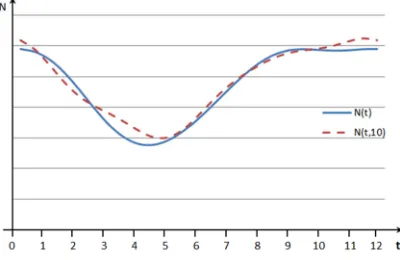
[image:7.612.316.512.423.719.2]

Comparative charts of calculations are presented in figures 4 and 5. Horizontal axis reflects time per hour. N(t,10)− reflects the approximation of N(t) functions over 10 iterations. N(t,20)− means the approximation of N(t) functions over 20 iterations.

Figure 4:Result of N(t) function approximation

[image:7.612.314.514.424.554.2] [image:7.612.92.298.473.619.2]

(8)

1396 The results of numerical experiment, depicted on the graphs, indicate a good level of approximation of generalized soil heat conductivity parameter, calculated with the use of the method developed, in relation to the values, acquired from the practical experiment.

6. CONCLUSIONS

The following results were obtained:

1) Based on the equations of heat conductivity the conjugate differential problem is built.

2) Supposing that the coefficient of overall heat conductivity is given in form of

∑

=

   



 ₊

+

= 4

1 0

12 cos ) ( 12 sin ) ( )

(

k

c s

t k k N t k k N N

t

N π π ,

iteration formulas of calculating for the coefficients of N(t)functions are worked out:

(

( , ; ) ()

)

( , ) ( ), )

( ) 1 (

0 0

max

n dt t H t T n t H

n N n N

t

g ψ β

θ − ⋅

+

+ =

+

∫

(

( ,; ) ()

)

( , ) , 12

sin ) , (

) , ( ) 1 , (

max

0

n k N n k N

g t

s

s s

ψ θ

π

β −

+

+ =

+

∫

(

( ,; ) ()

)

( , ) , 12

cos ) , (

) , ( ) 1 , (

max

0

n k N n k N

g t

c

c c

ψ θ

π

β −

+

+ =

+

∫

where k = 1,2,…4, n– number of iteration.

3) Using a programme written in C++, numerical calculations are conducted. The results of numerical calculations are shown in diagrams fig.1 - fig.5. Analysis of the above mentioned figures confirms that constructed iteration diagram results in a good convergence.

Numerical methods of solution and developed approach to calculation and theoretical model, implemented within the work, expands the theory of soil thermal behavior prognosis, the theory of non-linear differential schemes and the theory of coefficient reverse problem of heat distribution in soil.

The developed methods of calculating the coefficient of soil thermal conductivity and the differential schemes constructed can be applied to

solving certain problems of soil thermal behaviour prognosis, emerging in practice and during the process of production.

The developed calculation methods allow to create a device, fit for defining soil thermal conductivity coefficient, applied in-field, possessing relatively high accuracy of measurement and capable of non-destructive monitoring.

7. ACKNOWLEDGEMENT

The authors would like to thank Doctor Of Physical and Mathematical Sciences Bolatbek Rysbaiuly and Doctor of Technical Sciences Adamov Abilmazhin for discussion on the subject of this paper. They would also like to thank the referees for their suggestions.

REFERENCES

[1] J. A. Morrison and P. R. Norton: The heat capacity and thermal conductivity of apollo 11 lunar rocks 10017 and 10046 at liquid helium temperatures. Journal of Geophysical Research. Volume 75, Issue 32, 1970, pр. 6553–6557.

[2] Chudnovsky А.F. Thermo-physical characteristics of dispersive materials. State publishing of physics and mathematics literature. Moscow, 1962.

[3] G.S. Chichua: Thermo-physical characteristics of basic soil types of Georgian SSR. Autoabstract of doctoral thesis. Moscow, 1967.

[4] K.Ya. Kondratyev: Actinometry. Hydrometeorological publishing. Leningrad, 1965.

[5] D.A. de Vries: Some remarks on heat transfer by vapour movement in soil. Transactions 4th Int. Cong. Soil Sci., Vol. 2, Amsterdam, 1950, pp. 38-41.

[6] O. Krischer und H. Rohnaeter: Wärmeleitung und dampfdiffusion in feuchten gütern, VDI-Forschungsheft, 402, 1940.

[7] N.F. Bondarenko: Physics of underground water motion. Hydrometeorological publishing. Leningrad, 1973.

[8] А.I. Budagovsky: Soil moisture vapourising. “Science” publishing. Moscow, 1964.

[9] А.V. Lykov: Thermal and mass exchange. “Energy” publishing. Moscow, 1972.

(9)

1397 [11] А.А. Samarsky: Theory of differential

systems. “Science” publishing. Moscow, 1983.

[12] О.А. Geraschenko and В.G. Feodorov: Heat and temperature measurements. “Naukova dumka” publishing. Kiev, 1965.

[13] О.М. Alifanovв, Е.А. Artykhin and С.V. Rumyantsev: Extreme methods of solving incorrect problems. “Science” publishing. Moscow, 1988.

[14] М.М. Lavrentyev, V.G. Romanov and S.P. Shishatsky: Incorrect problems of mathematical physics and analysis. “Science” Publishing. Moscow, 1980.

[15] J. Beck, B. Blackwell and Ch. Saint-Claire: Incorrect reverse problems of heat conductivity. «Mir» publishing. Moscow, 1989.

[16] B.Rysbaiuly: Newton’s method to solve the problem of heat transfer in the freezing soil. Pensee Journal. Volume 76, Issue 1. Paris, 2014, pp. 261-275.

[17] A. Hasanov: Simultaneous determination of source terms in a linear parabolic problem from the final overdetermination: Weak solution approach. J. Mathematical Analysis and Applications. 330 (2007), рр. 766–779. [18] B. Rysbaiuly and A. Baimankulov: