Simultaneous Evolution of Architecture and Connection
Weights in Artificial Neural Network
G. V. R. Sagar
Assoc. Professor, G.P.R. Engg. College. Kurnool AP, 518007, India.S. Venkata Chalam
,
Ph.D Professor,CVR Engg. College, Hyderabad AP, India
ABSTRACT
The important issue for Designing architecture isthe evolution of Artificial Neural Network (ANN). There is no systematic method to design a near-optimal architecture for a given application or task. The pattern classification methods are used to design the neural network architectures and efforts towards the automatic design of network topologies, constructive and destructive algorithms can be used. In the proposed work the optimization of architectures and connection weights uses the evolutionary process. A single-point crossover is applied with selective schemas on the network space and evolution is introduced in the mutation stage so that an optimized ANNs are achieved.
Keywords: Artificial neural network, topology mutation,
schema theory1. INTRODUCTION
Designing architecture is an important issue in the evolution of ANN. Constructive and destructive algorithms can be used [1] in design of network architectures. The constructive algorithm begins with a small network, and hidden nodes, layers and connections are added to the network dynamically [2], but in the destructive algorithm starts with large network and hidden nodes and connections are deleted to construct the network dynamically [3]. The above two algorithms are called as incremental and decremental algorithms. Yao [4], has pointed out that the performance method of equation, MSE, Learning speed, reduced complexity about architectures are represented as a search problem in the architecture space. Each performance level of all these, forms a surface in the architecture design space. Finding the optimal architecture design is the highest point on this surface. There are several surface methods considered by using EAs for finding the best network topology which gives the better solution rather than incremental and decremental algorithms. Network topology characteristics presented by miller [5] refer to the surface of possible solutions.
2. ENCODING METHODS:
The efficiency of feed-forward network depends on the topology of the networks size and structures. The EAs have been used two major ways for searching network topologies
i) Direct encoding. ii) Indirect encoding.
2.1 Direct Encoding Method:
In this process the direct transformation of genotypes into phenotypes [8], [9] [17], [18], and the connection topology is represented by means of a adjacency matrix and many examples of this method are given in [5], [6], [10]. This encoding is easy to implement, but it does not scale well. As a consequence, the training the entire populations by using Back-Propagation method can be extremely slow.
2.2 Indirect Encoding Method:
The scalability problem in direct method will be overcome by this method. This method requires a considerable effort for neural network decoding. But sometimes, the network can be pre-structured architectures, which makes the search space is very much smaller. In this method some network parameters like number of layers, the size of the layers, the bias etc. may also defined for optimal architectures.The genetic programming [15], [16] has be changed in order to work with graph programming has to be changed in order to work with graph structures, So that ANNs can be developed, this also allowed the obtaining of simplified network that solve the problem with a small group of neurons. This system achieves good results. The drawback of this system has an over fitting problem
3. SIMULTANEOUS EVOLUTION OF
ARCHITECTURE AND WEIGHTS:
The ANNs structure optimization to tackle the effects of noisy fitness evolution problem is to consider mapping between genotypes and phenotypes of each individual [7]. This is possible by simultaneous evolution of connection weights and architecture of the network structures. This results the fully functioning network can be evolved without any intervention by an expert. The evolutionary genetic operators implemented in this work consider crossover as the predominant operator and mutation is defined as the secondary operator, only responsible for slight qualitative changes in the ANNs features. Neuro-evolutionary method using augmenting topologies (NEAT) was presented by Stanley and Mikkulainen [13], [14].4.
PROPOSED
EVOLUTIONARY
ARTIFICIAL NEURAL NETWORKS:
The evolutionary operators, discussed in [17] only Recombination (Crossover) and topology mutation are discussed here. In this work for an ANN optimization two types of activation functions are used to define the fitness evaluation, one is log sigmoid and other is tangent sigmoid activation functions.for each parent because the genotype lengths of individuals are variable. The cutting point is taken only between the one layer and the next layer (for two hidden layer between second layers of two network parents). A new evolutionary weight matrix has created to make connection between two layers at the cutting points in the parents producing the two off-springs, so that the population is maintained constant.
4.2 Topology Mutation:
The function of this operator is to introduce the new genetic information and to keep diversity in the population. The weight mutation is applied first given in [17], [11], [12]. Based on the concept of evolutionary algorithm, topological mutations are applied after evolution of weights. This mutation operator affects the network architecture size. This means that the number of neurons or nodes in each layer and number of hidden layers are changed. The mutation process uses the different activation functions. Based on the activation functions response, four types of architecture mutations are used they are insertion of a new hidden node, or a new hidden layer, elimination of hidden node or hidden layer.
4.3
Pseudo
code
of
Evolutionary
Architecture
and
connection
weights
algorithm:
% initialization of population
1. sz = total weights and architecture; 2. Fori = 1: popsize;
3. pop(i)=sz number of random number; 4. End
% Evaluating optimal connection weights
5. For j=1: popsize/2;
6. pickup two parents randomly through uniform distribution;
7 cp=weight cross over position defined by randomly pickup any active node position; 8. To create offspring, exchange all incoming weights to selectednodes cp between parents; 9. For each offspring;
10 place of mutation, mp = randomly selected active node;
11. For all incoming weights w to selected nodemp;
12. w=w+N (0, 1); 13. End
14. End
15. End
16. Optimal Connection weights
17. Use these connections to establish the ANN in the architecture space
% offspring population creation (Architecture)
18 An crossover of ANNs using single point method and assigningthe evolved
connection weights and activation functions. 19. For j=1: popsize/2;
20. pickup two parents randomly through uniform distribution
21. Train each ANN with decoded architectures by evolutionary
learning rule with optimized weights. 22. compute the fitness of each individuals based on the MSE.
23. Apply the search operator to the parents
and generate the off-springs.
24. To create offspring network exchange all second layer and output layer nodes
between two parent networks and assign the evolved weights to establish connections.
25. End
% Topology Mutation
26.For each offspring network;
27. place of mutation, am = randomly selected hidden active layer;
28. For all the neurons in the active layer find the neuron which is
not contributing to the network efficiently, delete the node and
duplicatethe highest efficientneuron in the same layer;
29. If layer contains less than one neuron delete the layer and add
thenew layer randomly with weight matrix in the same layer
30. End
31. End
32. End
33. Offspring population, off_pop available; 34. npop= [pop; off_pop];
% Define fitness of each solution, 35. Fori=1:2*popsize;
36. wt=npop(i); 37. an=npop(i);
38. applywt to ANN architecture to get error value;
39. ANNs to get error value; 40. define fitness as fit(i)=1/error; 41. End
% Tournament selection
42. Apply schema theory on Architectures and selects the schemata based on fitness
43. For r =1:2*popsize;
44. pick P number of Challengers in each schemata based on the fitness, where P = 10% of popsize;
45. arrange the tournament w.r.t fitness between schemata and selected P challengers.;
46. End
47. Arrange score of all solution in ascending order;
48. sp=pick up the best half score position ; 49. select next generation solution as solution corresponding to position sp;
50. repeat the process from step 5 until terminating criteria does not satisfy 51. final solution=solution with maximum fitness and minimum nodes and
connectionsin last generation.
5. EXPERIMENTAL SETUP:
10 independent trails have given to get the generalize behavior. Condition of terminating criteria is taken as fixed iteration and it is equal to 100 for EA. Table 5.1 gives all the parameters of the algorithm and default setting values are taken for considered problem.
5.1 Performance of N-Bit Parity (XOR)
classification Problem:
[image:3.595.315.530.75.197.2] [image:3.595.317.529.256.374.2] [image:3.595.317.530.423.544.2] [image:3.595.48.258.427.637.2]5.1.0 2-Bit parity classification Problem:
For 2-bit parity, all networks in the space has a maximum of 10 nodes including 2 inputs and 1 output node i.e. the size is [2 3 2 1 2]. This allowed for hidden layer configurations up to 5 nodes to be evolved. The average and best generation over all runs that found a solution for parity-2 using accuracy fitness function and the smallest architecture size found. The optimized network contains one hidden layer of two nodes with uni-model sigmoid activation function and all possible optimal connections between nodes. The mean square error (MSE) with minimum value over 10 trail runs is 1.3265e-18 and the performance of 5 runs are shown in Fig (1) and the run 3,4, & 5 completed in 50 generations and run1&2 completed in 20 generations.The average number of hidden nodes over 10 successful trail runs is 2.1 and the average number of connections is 7.9. Similarly, for 4-bit parity shown in Fig (2) the average number of hidden nodes over 10 trail runs is 2.3 and average number of connections is 14.7 with a minimum MSE is equal to 2.1219e-026.
Table: 5.1Default parameters.
FIGURE 1 Performance of Evolutionary ANN for 2-bit parity with initial sizes of [2 3 2 1 2].
FIGURE 2 Performance of Evolutionary ANN for 4-bit parity with initial size of [4 5 4 1 2].
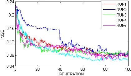
FIGURE 3 Performance of Evolutionary ANN for Pima India diabetes with initial size of [9 4 5 1 2].
Symbol Parameter Default
value
N Population size 20
Seed Previously saved population none
Probability of inserting a hidden
layer 0.1
Probability of deleting a hidden
layer 0.05
Probability of inserting a neuron
in hidden layer 0.05
Probability of deleting a neuron
hidden layer 0.05
Probability of crossover 0.1
Number of network inputs specific Prob.
Number of network outputs Prob. specific
The minimum mean square error value was found in the 5th trail and is equal to 2.1219e-026 for 2-bit parity and is equal to 9.2154e-026 for 4-bit parity has given in the Table 5.2.
5.2.0 Performance of Real-Time dataset
classification Problems:
In the real time dataset classification problems, only two classification problems are considered for result verification of the proposed algorithm. One is Pima India Diabetes and second one is the SPECT Heart dataset problems which were discussedin [8].
5.2.1 Pima India Diabetes:
The Training, Test and number of instance are discussed in [8]. The first 400 instances were used to process the training and the remaining 240 instances were used to test. The evolutionary process initialized with all the networks in the architecture space with an defend architecture size, example of size [9 4 5 1 2] i.e. 9 inputs, 4 hidden nodes in 1st hidden layer, 5 hidden nodes in second hidden layer, one output layer with one node and last digit 2 represents the number of layers (but the maximum number of hidden neurons allowed is (2N + 1)). After the evolutionary ANN process the optimized network consists of only 3 hidden nodes in a single hidden layer with uni-model sigmoid activation function and the result of the Pima India diabetes for ten trail runs are executed and the average percentage error values of the training and test process are summarized in Table 5.2 and 5 trail runs are shown in Fig (3) except trail 1 remaining all shows minimum mean square error. The average mean square error is 8.6214e-03.
5.2.2 SPECT Heart Classification problem:
The first 200 instances were used to process the training and the remaining 67 instances were used to test. The evolutionary process initialized all the network space with a defined structure an example architecture size of [14 4 5 1 2]. After the evolutionary ANN process the optimized network consists of only 3 hidden nodes in layer 1 and 2 hidden nodes in layer2 with all nodes contain the uni-model activation function
[image:4.595.102.495.84.218.2]The results of the heart dataset are as shown in Table 5.2 for ten trail runs are executed and the average percentage error values of the training and test process are summarized in Table 5.2 and 5 trail runs are shown in Fig (4) with an average mean square error of 7.7264e-003.
FIGURE 4 Performance of Evolutionary ANN for SPECT Heart dataset with initial size of [14 4 5 1 2].
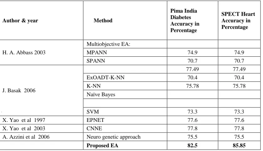
5.2.3 Comparison to the Literature:
In order to better validate the proposed work in this thesis, a comparison with a list of some, more recent works presented in the literature is given in the Table 5.3. All these works has used the Pima Indian Diabetes and SPECT heart problem as benchmark. The proposed EA approachcompares well with respect to the other works, obtaining good consistency and accuracy.
6. CONCLUSION:
Determination of optimal architecture and weights in ANN in the phase of learning has obtained by using the concept of evolutionary genetic algorithm. Proposed method of both architecture and weights adjustment has shown outperform at every level for 2-Bit, 4-bit parity compared to the fixed architecture back-propagation algorithm given in [17],[18] and in the case of real dataset classification problems an excellent percentage of accuracy is achieved with minimized network size.
Trail No.
2-Bit Parity 4-Bit Parity
MSE([2 3 2 1 2]) MSE([2 2 3 1 2]) MSE([4 5 4 1 2]) MSE([4 4 5 1 2])
1 9.0084e-003 4.6115e-006 3.2548e-006 6.2587e-014
2 2.1219e-026 9.4020e-028 1.3548e-002 7.6584e-005
3 2.0416e-014 9.6960e-032 6.3254e-011 9.4851e-021
4 1.3406e-003 6.0631e-037 5.4856e-019 1.9562e-019
5 2.1219e-026 6.9969e-019 9.2154e-026 1.7541e-003
6 9.0084e-003 4.6115e-006 9.3554e-004 6.4851e-006
7 2.1219e-026 9.4020e-028 2.8754e-014 5.9745e-023 8 2.0416e-014 9.6960e-032 9.2365e-013 4.1254e-016
9 1.3406e-003 6.0631e-037 3.4587e-001 5.4216e-014
10 3.2323e-022 6.9969e-019 8.2657e-016 8.6541e-020
[image:4.595.317.528.348.470.2]+
7. REFERENCES
[1] X.Yao. Evolving artificial neural networks. In Proceeding so on IEEE,pages 1423–1447, 1999.
[2] X.Yao and Y.Liu. Anew evolutionary system for evolving artificial neural networks. IEEE Transaction son NeuralNetworks,8(3):694–713,May1997.
[3] M.C.Mozeand P.Smolensky. Using relevance to reduce network size automatically.connectionScience,1(1):3–16, 1989. [4] X.Yao and Y.Liu. Towards designing artificial networks by
evolution.AppliedMathematicsandComputation,91(1):83– 90,1998
[5] G.F.Miller, P.M.Todd, and S.U.Hegde. Designing neural networks using genetic algorithms. In J.D.Schaffer, editor, ProceedingsoftheThirdInternationalConferenceonGeneticAlgor ithm,pages379–384,1989
[6] D.Whitley, T.Starkweather, and C.Bogart. Genetic algorithms and neural networks: Optimizing connections and connectivity. Parallel computing, 14:347–361, 1993.
[7] P.J.B.Hancock. Genetic algorithms and permutation problems: A comparison of recombination operators for neural net structure specification. In L.D.Whitleyand J.D.Schaffer, editors, Proceedings of the Third International Workshop on Combinations GeneticAlgorithmsNeuralNetworks,pages108– 122,1992GeneticAlgorithms,pages379–384,1989
[8] X. Yao and Y. Liu, “EPNet for chaotic time-series prediction,” in Select. Papers 1st Asia-Pacific Conf. Simulated Evolution and Learning (SEAL’96), vol. 1285 of Lecture Notes in Artificial Intelligence, X. Yao, J.H. Kim, and T.Furuhashi, Eds. Berlin, Germany: Springer-Verlag, 1997, pp. 146–156
Parameter Pima-India Diabetes data set SPECT Heart Data set
Number Of Runs 10 10
Number Of Generations 102 90
Number of Training patterns used 500 200
Average Training Set Accuracy 76.0 86.0
Number of Test patterns used 268 67
Average Test Set Accuracy 81.5 85.2
Initial Number of Hidden layers / Nodes 2 / [4 5] 2 / [4 5]
Final Number of Hidden layers / Nodes 1 / [2] 1 / [3]
Population size 50 50
Number of inputs 09 14
[image:5.595.74.508.108.256.2]Number of outputs 01 01
Table 5.2 Results of Real time dataset classifiers problems.
Table 5.3: Comparison of classification performance on the Pima India Diabetes and SPECT Heart problems
Author & year Method
Pima India Diabetes Accuracy in Percentage
SPECT Heart Accuracy in Percentage
H. A. Abbass 2003
Multiobjective EA:
MPANN 74.9 74.9
SPANN 70.7 70.7
J. Basak 2006
77.49 77.49
ExOADT-K-NN 70.4 70.4
K-NN 75.78 75.78
Naïve Bayes
SVM 73.3 73.3
X. Yao et al 1997 EPNET 77.6 77.6
X. Yao et al 2003 CNNE 77.8 77.8
A. Azzini et al 2006 Neuro genetic approach 75.5 75.5
[image:5.595.52.471.299.540.2][9] Y. Liu and X. Yao, “A population-based learning algorithmwhich learns both architectures and weights of neural networks,” Chinese J. Advanced Software Res., vol. 3, no. 1, pp.54–65, 1996.
[10]D. B. Fogel, “Phenotypes, genotypes, and operators in Evolutionarycomputation,” in Proc. 1995 IEEE Int.Conf. EvolutionaryComputation (ICEC’95), Perth, Australia, pp. 193–198.
[11]D. G. Stork, S. Walker, M. Burns, and B. Jackson, “Preadaptationin neural circuits,” in Proc. Int. Joint Conf. Neural Networks, vol. I, Washington, DC, 1990, pp. 202–205.
[12] D. White and P. Ligomenides, “GANNet: A genetic Algorithmfor optimizing topology and weights in neural network design, ”in Proc. Int. Workshop Artificial Neural Networks (IWANN’93),Lecture Notes in Computer Science, vol. 686. Berlin,Germany: Springer-Verlag, 1993, pp. 322–327.
[13] K.Stanley and R.Miikkulainen. Evolving neural networks through augmenting topologies. Evolutionary omputation,10(2):99–127,2002.
[14] K.O.Stanley and R.Miikkulainen. Efficient evolution of neural network topologies. In Proceeding of the Congress on Evolutionary Computation, CEC’02, pages1757–1762. IEEEComputerSocietyPress, 2002.
[15] Daniel Rivero, Julian Dorado, Juan R, and Rabunal, “Artificial neural Network Development by means of genetic programming with graph codification”, Proceedings of world academy of science, engineering and technology, Vol:15, pp 209-214, 2006. [16] Dario Floreano Æ Peter Du¨rr Æ Claudio Mattiussi , “
Neuro-evolution: from architectures to learning,” Springer-Verlag, January 2008.
[17] G.V.R. Sagar, et al. “Evolutionary Algorithm for Optimal Connection weights in Artificial Neural Networks,” IJE, vol. 5, Issue: 5, 2011.
[18] G.V.R. Sagar, S.V. Chalam “Evolutionary ANN Learning algorithm on Benchmark andReal time dataset Classification problems,” Current Development in Artificial Intelligence (CDAI), Aug 2012
![FIGURE 1 Performance of Evolutionary ANN for 2-bit parity with initial sizes of [2 3 2 1 2]](https://thumb-us.123doks.com/thumbv2/123dok_us/8103197.788550/3.595.317.530.423.544/figure-performance-evolutionary-ann-bit-parity-initial-sizes.webp)