31
Classification based Expert Selection for
Accurate Sales Forecasting
Darshana D. Chande
Computer Engineering Department, Government polytechnic, Thane
M.Vijayalakshmi
Information Technology department V.E.S.I.T, Chembur
ABSTRACT
Forecasting methods used in practice vary from domain to domain. This Paper focuses on sales forecasting. Most of the series considered here are composed of three components-Trend, seasonality and irregular. A series has been decomposed into its three components and multiple forecasters (Experts) have been applied on each component. Then these forecasters are recombined, using Cartesian product of their forecasts, to generate a set of Experts. A classification based scheme is proposed to identify a final good set of Experts which can be used in various combinations to create forecast for each series. Further it has been demonstrated that this forecasting system succeeds in producing a forecast that is more accurate than the Holt Winter method, which is a standard method of forecasting.
General Terms— Sales Forecasting, Times Series, Data Mining
Keywords--Decomposition, MAPE, Classification, Decision Tree, Experts, Combination
1.
INTRODUCTION
Sales forecasting is an important part of supply chain management. Timely and accurate sales forecasts are crucial in bridging the gap between supply and demand. So the selection and implementation of the proper forecast methodology is very important in sales forecasting. The primary goal of Time series forecasting is to improve the forecasting accuracy.
We have employed various kinds of pre-processing like decomposition. The series has been decomposed into multiple components such as Trend, seasonality and Irregular component. Each of these components is individually forecasted and their forecasts are combined back to come up with final forecast. The decomposition method has been used in which the component series has been built at each point with the help of some past points. Multiple forecasters are used and opinion is taken from their forecasts. For this the model is selected by determining the best model based on certain criteria and that model is used for combining. Combination Method is used, as a single model selection is associated with the instability problem [4] when limited data is available or when two or more models are performing well [17]. In such circumstances, a slight change in the data may result in the selection of different model. This inconsistency of model selection may result in high risk in final forecast.
Combining reduces the risk of forecasting. In our work we have used multiple Experts (forecasters) for forecasting individual component series, which gives multiple forecasts for each component. We then take Cartesian product of individual component forecasts which ultimately gives us a very large number of Experts (of the order of 105).The availability of such
a large number of Experts has enabled us to combine based on frequency and rank.
The outline of the paper is as follows. In Section 2, we present Literature Survey. In Section 3, we introduce our Decomposition followed by combining approach. We reviewed the basic forecasting models used here and some terms used in Data Mining relevant to this paper. In Section 4, the decision tree used in our algorithm is presented which shows the way we have classified the Experts. In Section 5, the Results are discussed; the study of effect of filtering out the poorly-performing forecasters is presented along with comparison with standard method. It also introduces a heuristic based on identification of the good and bad individual trend, seasonal and irregular component models derived from the classes of good and bad forecasters. A summary of our main results and conclusions are included in Section 6.
2.
LITERATURE SURVEY
There are two main approaches to forecasting- Quantitative methods (objective approach) and Qualitative methods (subjective approach).Quantitative forecasting methods are based on analysis of historical data and assume that past patterns in data can be used to forecast future data points. Qualitative forecasting techniques employ the judgment of Experts in specified field to generate forecasts. They are based on educated guesses or opinions of experts in that area. There are two types of quantitative methods: Time-series method and explanatory methods.
2.1 Time Series Introduction
A time series is a sequence of observations taken sequentially in time. It can be seen as being composed of three components: Trend (Change in the mean of time series), Seasonality (repetition of a particular pattern of observations after certain fixed time interval) and Irregular component (random noise). This calls for decomposition methods that will generate individual components series from the original series. These methods form one important part of the literature on forecasting. There exists various decomposition methods e.g. Holt-winter method, Exponential smoothing method, ARIMA etc. that are used to get these component series from the original series. Some of them are discussed in next section.
A time series can be broken down into its individual components. The decomposition of time series is a statistical method that breaks a time series down into its components (Trend, Seasonal, Cyclical, and Random).
2.2
Basic Time Series Methods
underlying trend, seasonal and cyclic components. Smoothing techniques are used to reduce irregularities (random fluctuations) in time series data. They provide a clearer view of the true underlying behaviour of the series.
Smoothing methods are Averaging Methods, Exponential smoothing methods, Box-Jenkins or ARIMA etc. Simple moving average takes certain number of past periods and adds them together; then divide by the number of periods. Simple Moving Averages (MA) is effective and efficient approach if the data is stationary. Exponential smoothing methods is a widely method used of forecasting based on the time series itself. An ES is an averaging technique that uses unequal weights; however, the weights applied to past observations decline in an exponential manner. Double exponential smoothing is better at handling trends. Triple Exponential Smoothing is better at handling parabola trends. Holt's linear exponential smoothing (LES) is an extension of simple exponential smoothing. This method is used when a series has no seasonality and exhibits some form of trend. This is an extension of exponential smoothing to take into account a possible linear trend. Other methods Hot-winter and ARIMA are discussed in next section.
2.3 Combination
Normally there are many forecasting methods (‘Experts’) available, and so one has to decide whether to select only a single Expert or to combine the forecasts of different Experts in some way to get the final forecast.
The forecast accuracy can be substantially improved through combination [3][16] of multiple individual forecasts. The reason behind this was assumed to be that one Expert could not entirely capture the details of underlying process but multiple Experts could capture different aspects of it and so should give better results. Moving to the methods used for decomposition and combining, lot of work has already been done [15].
2.4 Data Mining
Data mining is the process that attempts to discover patterns in large data sets. The overall goal of the data mining process is to extract information from a data set and transform it into an understandable structure for further use. The data mining step might identify multiple groups in the data, which can then be used to obtain more accurate prediction results.
2.5 Classification
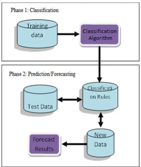
Classification is a data mining function that assigns items in a collection to target categories or classes. The goal of classification is to accurately predict the target class for each case in the data. A classification task (Figure 1) begins with a data set in which the class assignments are known. Classifications are discrete and do not imply order. The simplest type of classification problem is binary classification. In binary classification, the target attribute has only two possible values. Multiclass targets have more than two values.
In the model build (training) process, a classification algorithm finds relationships between the values of the predictors and the values of the target. Different classification algorithms use different techniques for finding relationships. These relationships are summarized in a model, which can then be applied to a different data set in which the class assignments are unknown.
[image:2.595.313.541.68.339.2]
Figure 1. Classification and Prediction Process
Classification models are tested by comparing the predicted values to known target values in a set of test data. The historical data for a classification project is typically divided into two data sets: one for building the model; the other for testing the model.
Classification problem is known as supervised learning, while clustering is known as unsupervised learning. Different classification algorithms are Decision trees, K-nearest neighbour algorithm, Neural networks [13], Memory (Case) based reasoning, Bayesian networks, Genetic algorithms etc.
2.6 Decision Tree
In data mining, a decision tree is a predictive model which can be used to represent both classifiers and Regression models. The decision tree refers to a hierarchical model of decisions and their consequences. The decision maker employs decision tree to identify the strategy most likely to reach the goals. When a decision tree is used for classification task, it is referred to as Classification tree. Classification trees are used to classify an object or an instance to a predefined set of classes based on their attributes. The use of decision tree is very popular technique in data mining. Decision trees are self-explanatory. They are usually represented graphically as hierarchical structures, making them easier to interpret than other techniques.
2.7 Challenges
33
3.
DECOMPOSITION
AND
COMBINING
A time series is a sequence of observations recorded at successive intervals of time. It is often the case that adjacent observations are dependent. These dependencies are captured by various time series models such as Holt Winter, ARIMA, etc.
Any time series is a composition of many individual underlying component time series. Some of these components are predictable whereas other components may be almost random which can be difficult to predict. Decomposing a series into such components enables us to analyse the behaviour of each component and this can help to improving the accuracy of the final forecast given by Brockwell [1],Makridakis [2]. A typical sales time series can be considered to be a combination of four components (i.e. trend component, cyclic component seasonal component, and irregular component).
The Seasonal component models patterns of change in a time series within a year. These patterns relate to periodic fluctuations of constant length, tend to repeat themselves each year. The Trend represents changes in the level of the series. The Cyclic component refers to patterns, or waves, in the data that are repeated after approximately equal intervals with approximately equal intensity, with period normally larger than seasonal period. Usually the trend and cyclic component are together treated as the Trend component. The Irregular component refers to variations not covered by the above components.
3.1 Decomposition model
Mathematical representation of the decomposition approach is: Where
Dt is the time series value (actual data) at period t. St is the seasonal component (index) at period t. Tt is the trend cycle component at period t.
ICt is the irregular (remainder) component at period t.
The decomposition could be additive if the magnitude of
seasonal fluctuations do not vary with the level of the series.
We have a multiplicative decomposition if seasonality fluctuates and increases and decreases with the level of the series.
Multiplicative model is more prevalent with economic series since most seasonal economic series have seasonal variation which increases with the level of the series. Further experiments carried out on a sample set of sales series has indicated that seasonal multiplicative model performs better than the additive model [15][20].In this research we shall thus use the multiplicative decomposition model. A method used in forecasting a single component is referred to as an atomic forecaster. A forecaster for the original series is a triplet made up of the atomic forecasters for each component. The set of such triplets is the Cartesian product of the sets of forecasters for the T, S and I components. Each such triplet of atomic forecasters (T, S, I) is called an “Expert”.
In this work, a total of 86 Trend models (atomic forecasters), 33 Seasonal models and 34 Irregular component models have been used. These are mostly ARIMA and seasonal ARIMA models of different orders. The Cartesian product of the Trend, Seasonal and Irregular models gives rise to 96,492 Expert forecasts per point. The Appendix includes a list of atomic
forecasters used in this work. Two of the best known methods of forecasting seasonal data (such as retail sales) are the Holt-Winter method and seasonal ARIMA which is briefly reviewed next.
3.2 Basic Forecasting Models
3.2.1 Holt-Winter Method
The Holt-Winter’s method [1] is used for the time series that has both trend and seasonal components. In addition to Holt parameters, suppose that the series exhibits multiplicative seasonality then HW method is used as by B. Menzes [15]and Venugopal [20]. Winters’ smoothing method can remove seasonality and makes long term fluctuations in the series stand out more clearly. There are two variants of this method, additive and multiplicative.
Multiplicative Seasonality
The seasonality is multiplicative [2][3] if the magnitude of the seasonal variation increases with an increase in the mean level of the time series. It is additive if the seasonal effect does not depend on the current mean level of the time series.
For multiplicative seasonality the updating equations are::
Where s is the number of periods in one cycle of seasons e.g. number of months or quarters in a year.
There are three smoothing parameters α, β, and γ which all must be positive and less than one.
To initialize we need one complete cycle of data, i.e. s values. Then set
To initialize trend we use s + k time periods.
If the series is long enough then a good choice is to make k = s so that two complete cycles are used. However we can, at a pinch, use k = 1.
Initial seasonal indices can be taken as
The parameters α, β, γ should lie in the interval (0, 1), and can be selected by minimising MAD, MSE or MAPE.
Additive Seasonality
The equations are
Where s is the number of periods in one cycle.
t t
t s mm t s t t t t t t t t t t s t t t
S
m
b
L
F
S
L
Y
S
b
L
L
b
b
L
S
Y
L
)
1
(
)
1
(
)
(
)
)(
1
(
1 1 1 1
) ... ( 1 2 1 ss Y Y Y
s
L
s k L Y S s k
k 1,2,...,
m s t t t m t s t t t t t t t t t t s t t t
S
m
b
L
F
S
L
Y
S
b
L
L
b
b
L
S
Y
L
)
1
(
)
(
)
1
(
)
(
)
)(
1
(
)
(
1 1 1 1
) (1 1 1 2 2
s y y s y y s y y s
b s s ss s
The initial values of Ls and bs can be as in the multiplicative case. The initial seasonal indices can be taken as
The parameters α, β, γ should lie in the interval (0, 1), and can again be selected by minimising MAD, MSE or MAPE.
3.2.2 Autoregressive Integrated Moving
Average (ARIMA)
The Autoregressive Integrated Moving Average (ARIMA) models [1][2], or Box-Jenkins methodology, are a class of linear models that is capable of representing stationary as well as nonstationary time series. ARIMA methodology of forecasting is different from most methods because it does not assume any particular pattern in the historical data of the series to be forecast.
Models for time series data can have many forms. When modelling variations in the level of a process, three broad classes of practical importance are the autoregressive (AR) models, the integrated (I) models, and the moving average (MA) models. These three classes depend linearly on previous data points. Combinations of these ideas produce autoregressive moving average (ARMA) and autoregressive integrated moving average (ARIMA) models.
Seasonal ARIMA models a pattern that repeats seasonally over time. It is classified as an ARIMA (p,d,q)x(P,D,Q) model, where
P is the number of seasonal autoregressive (SAR) terms, D is the number of seasonal differences,
Q is the number of seasonal moving average (SMA) terms Non Seasonal ARIMA Models are classified as an "ARIMA (p,d,q)" model, where:
p is the number of autoregressive terms, d is the number of non seasonal differences, and
q is the number of lagged forecast errors in the prediction equation.
4.
THE
PROPOSAL
We are using Classification method of Data Mining for forecasting the time series. All our hypotheses are tested on real life monthly sales series from standard library (Table 6). We use the method of decomposition and combining to get the final forecast.
4.1 Preliminaries
Our proposal uses decomposition as pre-processing. After decomposing the given time series, we use 86 Trend Experts, 33 seasonal Experts, 34 irregular Experts. Their Cartesian product gives us around 100000 forecasts and their combination gives the final forecast. Model combining has been explored in several papers [9][16].
Our experiments are performed on about 25 series taken from the Time Series Library [19] and the Economic Time Series Page [18][19]. The series represent monthly sales data over 10 – 15 years of diverse items such as wine, beverages, jewellery, gasoline and single family homes. They capture the vagaries often encountered in demand sales series. Abraham is highly regular, Dry is less so, Hsales exhibits a low-frequency cyclical nature and Sweet has highly anomalous behaviour in the mid-section. For demand sales, the most widely used error method for a forecasting model/method is the Mean Absolute Percentage Error (MAPE) defined by
Here
is the forecast of point and is the actual value at point.
4.2 Classification Based Forecasting
The Decision Tree method of classification [5][12][14] has been used to categorise the models. Firstly APE values calculated for all the models and after sorting on APE value, top 20000 models are selected as Good and bottom 20000 as Poor performer and divided them in different classes considering their frequency and rank. The criteria used for classification is shown in the tree (Figure 2).
Discarded: Discarded: Not used for Not used for Further Processing further Processing
Class Label: BAD
Class Label: BEST Class Label: GOOD
Class Label: EXCELLENT
Figure 2. Decision Tree
4.3
The Basic Algorithm / Pseudo code
Let ‘n’ be the total number of points in the series.
We use the first ‘n1’ points to learn one or more sets of good Experts and then use these to forecast the last ‘n2’ points of the series.
Total input: 96492(86*34*33) models
Sample taken: Top and Bottom, 20000 of 96492(After Sorting on MAPE)
We have n=96492, n1=20000, n2=24
Training Phase:
For each point, t, of the series between i = 1 to n
Identify the top n1 Experts and bottom n1based on their MAPE Then find out the frequency of each Expert in the set of top 20000
Also calculate Rank for each Expert
Then using Decision tree algorithm, based on Rank and frequency identify the BEST, Good and Bad Experts as per the applied condition
Find out the MAPE for these Experts
In the next step find out those Experts which survive after filtering Best
These are the Excellent (Ei) Experts which gives min. MAPE for most of the series
s k
L Y
Sk k s 1,2,...,
96492 forecasts generated by combining 86*34*33(TSI) Experts
All Experts in Good (min. APE) 20000 Forecasts
All Experts in Bad (max.APE) 20000 Forecasts
Experts having Count > avg.-1%
Experts having Count <= avg.-1%
quote
from
the
docume
nt or
the
summar
y of an
interesti
ng
point.
You
can
position
the text
box
anywhe
re in the
docume
nt. Use
the
Drawin
g Tools
tab to
change
the
formatti
ng of
the pull
quote
Experts having Count > avg.
Experts having Count <= avg.
Rank>10200 Rank<=10200
35 Denote these sets of Experts E1, E2, etc
Choose the Ei with the best MAPE for forecasting in the testing phase.
Testing Phase:
For each point, t in the interval comprising the last n2 points of the series
Compute the forecast for point t of each Expert in the set E Compute the mean of these |E| forecasts as the forecast at point t
Compute MAPE for the last n2 points.
5. DISCUSSION OF RESULTS
Multiple Experts have been used for the sales series and also for the individual components of the series obtained after applying basic decomposition. The models considered for constructing the Expert are ARIMA (including Seasonal ARIMA) models of various orders and various Exponential Smoothing Models such as Holt Winter Model, Holt Model, Seasonal Exponential Smoothing, Etc in SPSS Tool. Some Appropriate transformation like logarithmic transformation is often used for time series that show exponential growth or variability proportional.
Then Cartesian product of all components is done to get the final forecast. In this way we have 86*34*33= 96492 forecast for each point of data. Finally, we have selected 20000 best (min APE) forecast with their Expert ids as the final dataset for Best and Good models and 20000 (max APE) forecasts with their Expert ids as final dataset for Bad models classification. Based on frequency of model appeared we calculated count and also a rank.
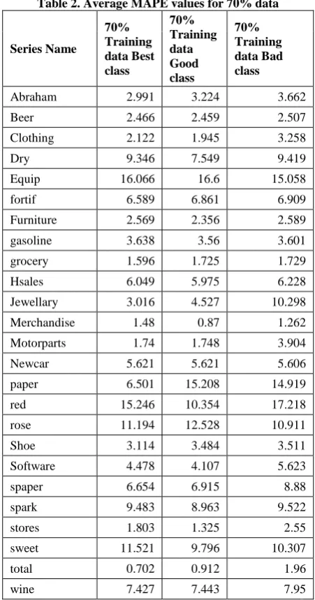
Then a classification of series has been done by applying Decision tree algorithm on 50% and 70% of data as training data and form Best, Good (from top 20000) and Bad(from bottom 20000) classes. The average values of MAPE for 50% and 70% data are given in the Table 1.
[image:5.595.308.537.67.763.2]
Table 1. Average MAPE values for 50% data
Series Name
50% Training data Best Class
50% Training data good class
50% Training data Bad class
Abraham 2.999 3.22 3.473
Beer 2.475 2.465 2.504
Clothing 2.028 2.019 3.262
Dry 9.466 7.55 8.381
Equip 15.409 16.87 15.748
Fortif 6.612 6.862 6.63
Furniture 2.582 2.345 2.583
gasoline 3.648 3.555 3.667
grocery 1.629 1.711 1.847
Hsales 6.114 5.982 6.226
Jewellary 3.03 4.552 5.761
Merchandise 0.932 0.892 1.284
Motorparts 1.57 1.772 3.9
Newcar 5.674 5.569 5.873
Paper 6.522 14.107 13.984
Red 14.827 10.32 17.199
Rose 11.49 12.605 10.909
Shoe 3.112 3.497 3.53
Software 5.291 4.126 5.107
Spaper 6.651 6.896 8.396
spark 9.701 8.917 9.345
stores 2.082 1.325 2.458
sweet 11.664 9.805 10.083
total 0.672 0.875 1.962
[image:5.595.312.538.278.708.2]wine 8.045 7.398 7.931
Table 2. Average MAPE values for 70% data
Series Name
70% Training data Best class
70% Training data Good class
70% Training data Bad class
Abraham 2.991 3.224 3.662
Beer 2.466 2.459 2.507
Clothing 2.122 1.945 3.258
Dry 9.346 7.549 9.419
Equip 16.066 16.6 15.058
fortif 6.589 6.861 6.909
Furniture 2.569 2.356 2.589
gasoline 3.638 3.56 3.601
grocery 1.596 1.725 1.729
Hsales 6.049 5.975 6.228
Jewellary 3.016 4.527 10.298
Merchandise 1.48 0.87 1.262
Motorparts 1.74 1.748 3.904
Newcar 5.621 5.621 5.606
paper 6.501 15.208 14.919
red 15.246 10.354 17.218
rose 11.194 12.528 10.911
Shoe 3.114 3.484 3.511
Software 4.478 4.107 5.623
spaper 6.654 6.915 8.88
spark 9.483 8.963 9.522
stores 1.803 1.325 2.55
sweet 11.521 9.796 10.307
total 0.702 0.912 1.96
wine 7.427 7.443 7.95
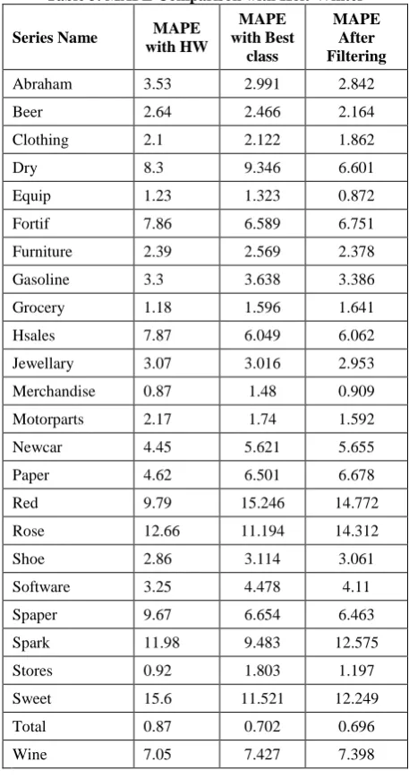
Finally the Best model has been filtered and Bad models have been removed, the models which survived after filtering are put in the class Excellent and which gave minimum MAPE for most of the series. MAPE comparison with Holt winter is shown in the Table 3 and the result was 7.17% improvement over the standard Holt-winter method. Table 4 shows improvement of MAPE over Holt-Winter.
Table 3.MAPE Comparison with Holt-Winter
Series Name MAPE with HW
MAPE with Best
class
MAPE After Filtering
Abraham 3.53 2.991 2.842
Beer 2.64 2.466 2.164
Clothing 2.1 2.122 1.862
Dry 8.3 9.346 6.601
Equip 1.23 1.323 0.872
Fortif 7.86 6.589 6.751
Furniture 2.39 2.569 2.378
Gasoline 3.3 3.638 3.386
Grocery 1.18 1.596 1.641
Hsales 7.87 6.049 6.062
Jewellary 3.07 3.016 2.953
Merchandise 0.87 1.48 0.909
Motorparts 2.17 1.74 1.592
Newcar 4.45 5.621 5.655
Paper 4.62 6.501 6.678
Red 9.79 15.246 14.772
Rose 12.66 11.194 14.312
Shoe 2.86 3.114 3.061
Software 3.25 4.478 4.11
Spaper 9.67 6.654 6.463
Spark 11.98 9.483 12.575
Stores 0.92 1.803 1.197
Sweet 15.6 11.521 12.249
Total 0.87 0.702 0.696
[image:6.595.55.284.163.598.2]Wine 7.05 7.427 7.398
Table 4. MAPE Improvement over Holt-Winter
Series Name
MAPE with HW
MAPE After Filtering
%
Improvement over HW
Abraham 3.53 2.842 19.477
Beer 2.64 2.164 18.02
Clothing 2.1 1.862 11.34
Dry 8.3 6.601 20.474
Equip 1.23 0.872 29.101
Fortif 7.86 6.751 14.113
Furniture 2.39 2.378 0.496
gasoline 3.3 3.386 -2.619
Hsales 7.87 6.062 22.971
Jewellary 3.07 2.953 3.819
Merchandise 0.87 0.909 -4.462
Motorparts 2.17 1.592 26.658
Newcar 4.45 5.655 -27.078
rose 12.66 14.312 -13.05
Shoe 2.86 3.061 -7.015
Software 3.25 4.11 -26.466
spaper 9.67 6.463 33.16
spark 11.98 12.575 -4.97
sweet 15.6 12.249 21.479
total 0.87 0.696 19.943
wine 7.05 7.398 -4.935
7.165
Bad performing series
grocery 1.18 1.641 -39.1
paper 4.62 6.678 -44.542
red 9.79 14.772 -50.886
stores 0.92 1.197 -30.129
37
[image:7.595.55.296.106.716.2]Table 5. Results of Filtering Models-Dry SeriesError! Not a valid link.
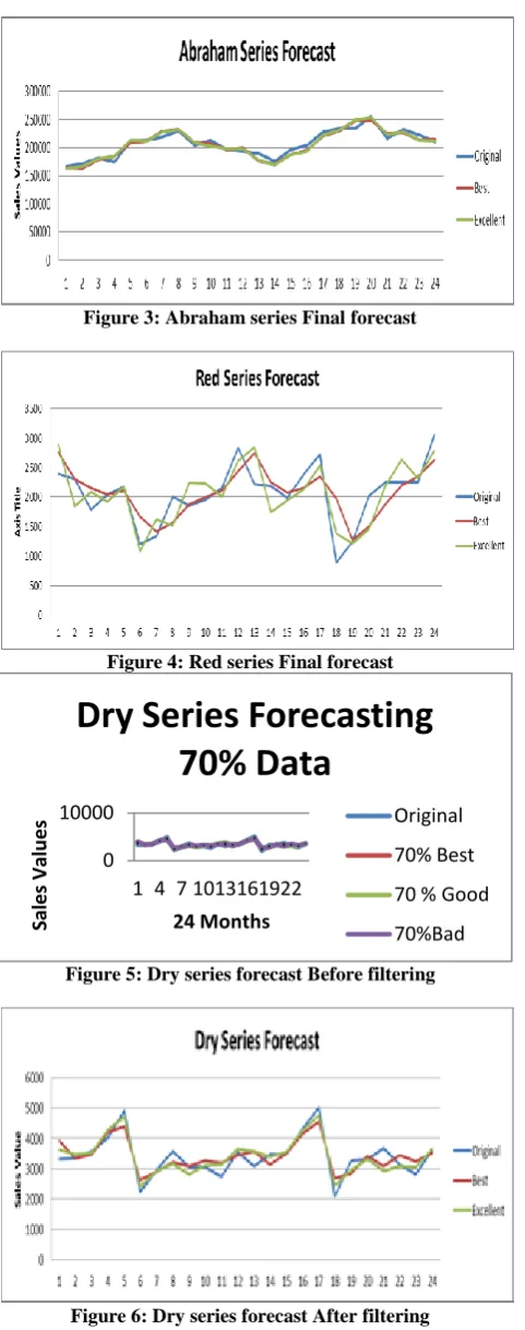
Figure 3: Abraham series Final forecast
Figure 4: Red series Final forecast
Figure 5: Dry series forecast Before filtering
Figure 6: Dry series forecast After filtering
6.
SUMMARY
AND
CONCLUSIONS
Combining models for sales forecasting helps reducing the risk involved in trusting a single forecast and improves forecasting
accuracy on average. The challenge lies in being able to select a set of consistently good models for a series. We zoomed in on the T, S and I component models comprising each good Expert at a point and identified the frequently occurring T, S and I models at each point. The Decision Tree method of Classification has been applied on the sets for each component yielding the good sets, T, S and I. After classifying the Best models, the product of the averages of the forecasts of the models in T, S and I were used as the final forecast (since we have used a multiplicative model of time series decomposition).
We studied two approaches. In the first, we identified a good set of Experts over a training period using both 50% and 70% of training data and used these Experts to forecast the series in the test phase (last 24 points of a series). The other approach is to identify a set of poorly performing forecasters and filter these from the total pool of Experts. The resulting set is used to forecast the series in the test phase. These results indicate that the later approach yields lower MAPE.
These approaches yield sufficient improvements of about 7.17% over Holt-Winter forecasting .As in the Table 4.
7.
ACKNOWLEDGEMENT
[image:7.595.307.545.359.754.2]We would like to thank our college and Principal for sponsoring us for the Higher education.
Table 6. Description of various Time Series
Series Name Description
abraham Monthly gasoline demand (Ontario gallon millions)
beer US retail sales: beer, wine liquor stores
clothing US retail sales: Clothing Stores
Dry Monthly Australian sales of dry white wine (Thousands of litres)
Equip
US retail inventories: Building materials, Garden equipment,
supply stores (Million Dollars)
fortif Monthly Australian sales of fortified wine
furniture US retail sales: Furniture Stores
gasoline US retail sales: gasoline station
grocery US retail sales: Grocery Stores
hsales Monthly sales of new one-family houses sold in the USA.
jewellary US retail sales: Jewellery Stores
merchandise US retail inventories: General merchandise stores
motorparts US retail inventories: motor vehicles and part dealers
newcar US retail sales: New car dealers
paper Monthly sale of printing and writing paper.
Red Monthly Australian sales of red wine
Rose Monthly Australian sales of rose wine
shoe US retail sales: Shoe stores
software US retail sales: Computer and software stores
spaper CFE specialty writing papers monthly sales
spark Monthly Australian sales of Sparkling wine
stores US retail inventories: Department stores (million dollars)
sweet Monthly Australian sales of sweet wine
total US retail inventories: total
wine Monthly Australian sales of wine 0
10000
1 4 7 10 13 16 19 22
Sal
e
s Val
u
e
s
24 Months
Dry Series Forecasting
70% Data
Original
70% Best
70 % Good
8. REFERENCES
[1] Brockwell, P.J. and Davis, R.A. (1991) Time series: Theory and Methods, 2ndEdn. Springer International Edition.
[2] Makridakis, S., Wheelwright, S., and Hyndman, R. (1998), Forecasting methods and Applications, 3rd Edition. Wiley: NY.
[3] Armstrong J. Scott, (2001), Combining Forecasts. Principles of Forecasting: A Handbook for Researchers and Practitioners, J. Scott Armstrong (ed.): Norwell, MA: Lower Academic Publishers.
[4] Bates, J. M., & Granger, C. W. J. (1969). Combination of forecasts. Operations Research Quarterly, 20: 451–468.
[5] “Performance comparison of Rule based Classification Algorithm” Prafulla Gupta, Durga Tosniwal, International Journal of Computer Science & informatics,Vol –I, 2011
[6] “Time-Series Classification based on Individualised Error Prediction” Krisztian Buza, Alexandros Nanopoulos, Lars Schmidt, 2010 13th IEEE International Conference on Computational Science and Engineering.
[7] Granger, C., & Ramanathan, R. (1984), Improved methods of combining forecasts, Journal of Forecasting 3:197–204.
[8] Hand, D. J. (2009). Mining the past to determine the future: Problems and possibilities. International Journal of Forecasting, 25(3), 441–451.
[9] Clemens Robert T. (1989), Combining forecasts: A review and annotated bibliography, International Journal of Forecasting 5: 559-583.
[10] YaohuiBai, Jiancheng Sun, JianguoLuo and Xiaobin Zhang “Forecasting Financial Time Series with Ensemble Learning”, 2010 International Symposium on Intelligent Signal Processing and Communication Systems (lSPACS 2010) December 6-8,2010 IEEE
[11] “Learning Weights for Linear Combination of Forecasting Methods”, Ricardo B. C. Prudencio and Teresa B. Ludermir, Proceedings of the Ninth Brazilian Symposium on Neural Networks (SBRN'06)0-7695-2680-2/06 $20.00 © 2006
[12] “Joint Segmentation and Classification of Time Series Using Class-Specific Features”Zhen Jane Wang and Peter Willett, Fellow, IEEE, ieee transactions on systems, man, and cybernetics—part b: cybernetics, vol. 34, no. 2, april 2004
[13] “The comparative study on linear and non-linear forecast-combination methods based on neural network” Han Dongmei1,2, Niu Wen-qing1, Yu Changrui1,, 1-4244-1312-5/07/$25.00 © 2007 IEEE
[14] “Wind Power Ramp Events Classification and Forecasting: A Data Mining Approach” Hamidreza Zareipour, Dongliang Huang, William Rosehart, , 978-1-4577-1002-5/11/$26.00 ©2011 IEEE
[15] Menezes B., Seth A., and Singh R., (2007), Can a million Experts improve your sales’ forecasts? European Symposium on Time Series Prediction, Helsinki, Finland, Feb. 7-9, 2007
[16] Zou H. and Yang Y., (2004), “Combining time series models for forecasting” International Journal of Forecasting, 20 (1): 69-84.
[17] Timmermann, A. (2006), “Forecast Combinations,” in eds. G. Elliott, C.W.J. Granger and A. Timmermann, Handbook of Economic Forecasting, Elsevier Press.
[18] Economagic.com: Economic time series page. http://www.economagic.com/.
[19] http://datamarket.com/data/list/? q=provider:tsdl granularity:monthly