Approaches of Self Localization in Wireless Sensor Networks and Directions in 3D

Approaches of Self Localization in Wireless Sensor

Networks and Directions in 3D

S. B. Kotwal

SMVD University, Katra, J&K-182320 India

Shekhar Verma

IIIT, Allahabad UP-211012 India

R.K. Abrol

SMVD University, Katra, J&K-182320 India

ABSTRACT

For variety of applications of sensor networks like tracking, monitoring, intrusion detection, geographical routing etc, localization plays a critical role. Any information from a remote node without its location is of less use in most of these applications. For small sized nodes with limited resources and densely distributed nodes, accurate and low cost localization is a critical issue. An efficient localization scheme exploits inherent collaborative nature of nodes in a sensor network to identify the location of nodes. More than 50 localization schemes exist as of now. Contribution of this study is to present various localization schemes based on various measurement techniques and algorithms thereof. Based on factors like accuracy, communication cost and feasibility in three dimensional scenarios is discussion. The comparison of these techniques can serve as direction for future research.

Keywords

Review Localization, 3D Localization.

1.

INTRODUCTION

Location identification or Localization in Wireless Sensor Networks (WSN) refers to creation of a map of a WSN by determining the geographical coordinates of each and every node. Location identification in WSN plays an important role in number of applications of WSN like:

1.1

Target Tracking

Sensors are deployed in the region which sense signals from the moving target. Using these sensed signals, the range, speed and direction of the target can be monitored.

1.2

Environmental Monitoring

A wireless sensor network can be used to detect the movements of soil during a landslide. The information about landslide will be useless unless tagged with location. If WSN nodes are deployed in forest any event of forest fire can be detected and its rate of spreading can also be calculated. Once again localization becomes necessary.

1.3

Intrusion Detection

In a scenario where it is not feasible or practical to implement manned surveillance and intrusion detection, un-manned, unattended detection is helpful. The wireless nodes capable of communicating with each other and using one or multiple of sensors like body heat, pressure, sound, light, electro-magnetic field, vibration, etc. can collectively detect and report any intrusion in the classified area. In this scenario since the nodes are deployed without any prior information of their placement, localization becomes the first step in the formation of the whole network. Once again localization becomes necessary.

1.4

Fleet

Monitoring

and

Rescue

Operations in battlefield

Using GPS modules on board of very few nodes, it is possible to identify the location of all member of the fleet wearing motes. A mote gathers its position by information exchange with other similar motes or via the GPS module equipped node, and reports its coordinates so that the location is tracked in real-time. The nodes can be equipped with sensors like temperature, humidity etc to avoid any disruption of the cold chain, helping to ensure the safety of food, pharmaceutical and chemical shipments. A soldier in the battlefield can also be located using this scheme.

All these applications require information about physical location of sensor nodes in the network. The other advantages of location identification in WSN are:

 Geographical Data Packet Routing,

 Collaborative Information and Signal Processing ,

 Saving the size of Data Packet by replacing Node ID by its Coordinates.

2.

LOCALIZATION PROBLEM

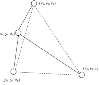
In a WSN of thousands of nodes in a WSN, it is not feasible to place nodes while recording their locations one by one. For example a network consisting of 1000 nodes will require around 17 hours to localize whole network assuming 1 minute required for placement of each node while recording its location. Whenever some event is triggered, sensed or measurement crosses the preset, the relevant information is communicated to the sink node from the sensor node. But this information is incomplete without location and time added to it by the sensor node, therefore location identification of every node in a WSN plays very important role to make the information useful. A WSN may consist of several nodes with (x, y, z) coordinates as shown in fig-1.

Considering the WSN consisting of M wireless nodes, where M=K+N. K being the no. of nodes with known their location in advance and are termed as anchors while N is the no. of nodes still unaware of their location. The locations of K nodes are [ 𝑥1, 𝑦1, 𝑧1 , 𝑥2, 𝑦2, 𝑧2 , … … . . (𝑥𝑘, 𝑦𝑘, 𝑧𝑘)] .

The problem is to determine the location of all other nodes as [ 𝑥𝑘+1, 𝑦𝑘+1, 𝑧𝑘+1 , 𝑥𝑘+2, 𝑦𝑘+2, 𝑧𝑘+2 , … … . . (𝑥𝑚, 𝑦𝑚, 𝑧𝑚)]

without human interference with accuracy (limit decided by the application) and low cost of communication.

The major factors which define performance of a localization scheme are its accuracy and efficiency.

Secondly GPS hardware typically uses more power than a sensor node as a whole which is likely to consume fair share of energy resource available on a small sized node, which will eventually reduce the life of a node. Lastly GPS based localization is not a good solution for indoor localization as direct link to GPS satellites would be required which is missing indoors. Therefore some scheme of localization needs to be developed which can work for outdoors and indoors as well.

3.

RELATED WORK

Several authors have presented the review of localizations algorithms for WSN. the authors in [1] and [2] focus on the security issues of localization techniques leaving other aspects as distance error, communication and energy costs involved in the localization process. Moreover, the secure localization is used in limited applications of WSN. In [3], the comparison is focused on the distance based algorithms. At present the comparison of angle or distance with angle based localization techniques is very limited. Only authors in [4] present a detailed review of the similar nature. Since then many new techniques have been proposed and the limitations of most of the then algorithms have been overcome by the latest versions of those algorithms. Depending upon application and deployment scenario, the localization may be required in three dimensional spaces rather than only two. Till year 2005, researchers were very little or not motivated to work in three dimensional localization. As per the knowledge of authors there is no review article present till date which covers review of three dimensional localization techniques. Therefore to attract research in the direction there is a need to present the latest and detailed review including comparison of modified and efficient version of older algorithms. Since most of the algorithms presented till date are the result of simulations on a MATLAB, OPNET, OMNET, etc. and very few of the techniques have really been implemented and tested on a real WSN, there is a need to identify techniques which can really be implemented in a WSN considering the architecture of WSN.

4.

LOCALIZATION PROCESS

The WSN initialization steps are shown below in figure-1.The localization process must be the initiated immediately after network formation for most of the applications of WSN so that any information after sensing some parameter can be tagged with location. Location estimation or localization is a two stage process as shown in fig-2. Firstly the measurement of distance, angle or connectivity is taken between nodes.

Secondly the algorithm based on measurement available is applied and approximate location of each node is recorded.

5.

MEASUREMENTS FOR

LOCALIZATION

A node in WSN requires two types of measurements for localization algorithm i.e. distance and/or angle w.r.t the other node in its communication range.

5.1

Distance

For distance only based localization schemes, at least three anchor nodes are required for localization of all nodes in a WSN, otherwise flip ambiguity. The Accurate distance measurement is a very tricky problem. At present, three distance measuring techniques are available:

5.1.1

Received Signal Strength (RSSI)

Once a node sends a fixed value of rf signal (in dBm) to other node with in communication range, the other node receives this signal with reduced intensity equal to𝑃𝑟 𝑑 𝑑𝐵𝑚 . The

relation between transmitted power and received signal can be found as below: IEEE 802.15.4 compatible Chipcon CC2420 transceiver operating in 2.4GHz ISM band is widely used in sensor nodes. A built-in received signal strength indicator of this transceiver gives an 8-bit digital value: RSSI_VAL. The power 𝑃𝑟 𝑑 𝑑𝐵𝑚 at the RF pins can be obtained directly

from RSSI_VAL using the following equation:

𝑃𝑟 𝑑 𝑑𝐵𝑚 = 𝑅𝑆𝑆𝐼_𝑉𝐴𝐿 + 𝑅𝑆𝑆𝐼_𝑂𝐹𝐹𝑆𝐸𝑇 (𝑑𝐵𝑚) – (ii)

Where 𝑅𝑆𝑆𝐼_𝑂𝐹𝐹𝑆𝐸𝑇 (𝑑𝐵𝑚) is approximately equal to -45 dBm [5].

Using most frequently used log normal shadow model [12], the relationship between the distance and RSSI value can be given as

𝑃𝑟 𝑑 𝑑𝐵𝑚 = 𝑃0 𝑑0 𝑑𝐵𝑚 − 10𝑛𝑝𝑙𝑜𝑔10 _𝑑𝑑

0 + 𝑋𝜎- (iii) Where𝑃𝑟 𝑑 𝑑𝐵𝑚 is the power received at distance d in

dBm, 𝑃0 𝑑0 𝑑𝐵𝑚 is the power received in dBm at a

reference distance𝑑0, 𝑛𝑝 refers to path loss exponent. The

value of 𝑛𝑝 depends upon surrounding environment, and typically lies between 2 to 6 [6].Because of various irregularities in RSSI as mentioned already, the error added in measured power is assumed to be zero mean Gaussian distributed variate and variance 𝜎. Assuming 𝐴 = 𝑃0 𝑑0 𝑑𝐵𝑚 + 𝑋𝜎, above equation becomes:

Fig-2. Localization Process

Lo

ca

li

za

ti

o

n

P

ro

ce

ss

Start

Take measurement

Apply Localization algorithm Network formation

Ready for sensing and routing Fig-1. WSN nodes in three dimensions

(𝑥3, 𝑦3, 𝑧3)

(𝑥1, 𝑦1, 𝑧1))

(𝑥2, 𝑦2, 𝑧2)

𝑃𝑟 𝑑 𝑑𝐵𝑚 = 𝐴 − 10𝑛𝑝𝑙𝑜𝑔10 _𝑑𝑑

0 - (iv)

The distance d between two nodes can be approximated by modifying above equation as:

𝑑 = 𝑑010{[𝐴−𝑃𝑟 𝑑 𝑑𝐵𝑚 ]/10𝑛𝑝} - (v)

Because of 𝐴 which is random in nature, there is a difference in the actual distance and approximated distance using above equation. Authors in [7] have done extensive experiment work for approximation using above technique and the standard deviation in range is shown to be approximately up to half of the actual range. In the non line of sight situation, error in distance estimation is worst. Therefore this method is applicable only in line of sight topologies.

5.1.2

Time of Arrival (ToA)

This approach uses a single packet sent from the one node to the other node containing the time it was transmitted, assuming there is perfect clock synchronization between the nodes. In such a scenario, the receiving node knows when the packet arrived and that it is synchronized with the sender node, the distance travelled can be calculated using the following formula:

𝑑 = 𝑐 ∗ ∆𝑡 - (vi)

Where d is the distance between the nodes, c is velocity of light and∆𝑡, the time difference. The advantage of using ToA is that it is not affected by channel fading, and is more accurate than RSSI [8], but achieving synchronization between the nodes creates another issue. Therefore this method of ranging is not popular.

5.1.3

Time Difference of Arrival (TDoA)

In TDoA, distance measurement depends upon the difference in time between two waves reaching same of different destinations with following combinations:

a) Both at Radio frequency

b) One at radio and other at Ultrasonic frequency c) Both at Ultrasonic frequency.

Once the difference in the arrival of the waves at destination is known, that can be used to approximate the distance. There is a slight difference in the methods shown at a), b) and c). For example in a), one source sends same RF signal to two different nodes. These two nodes calculate the difference of time arrival of the signal and calculate the distance between themselves and source node. Further details regarding a) are in [9].

In b), two destination nodes are not required and one source sends RF and ultra sonic signal at same time. The node at distance d will receive these two signals with some time difference as the speed of RF signal is higher than ultrasound signal. This difference of time in the reception of two signals is calculated by the node at distance d and using this information, the distance can be calculated as:

𝑑 = ∆𝑡 ∗ 𝑆 -(v)

Where ∆𝑡 is the difference in time of reception of two signals and

𝑆 =_{𝑐1−𝑐2}𝑐1∗𝑐2 -(vi)

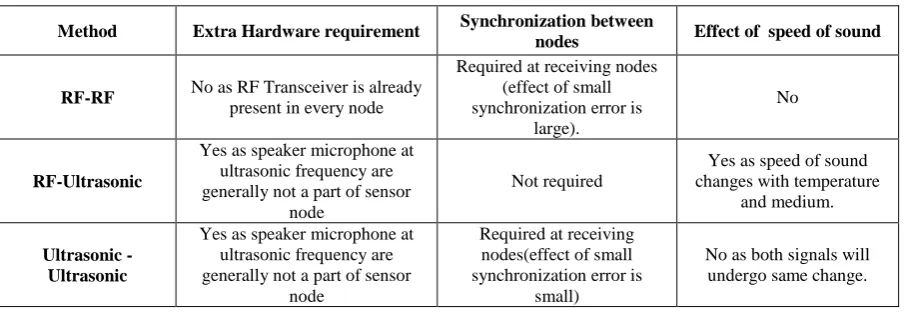
𝑐1 𝑎𝑛𝑑 𝑐2 are the speeds of RF and ultra sound signal. In c), the method is similar to a) but instead of RF signal; the signals used are ultrasound signals. A comparison of TDoA methods in a), b) and c) is given in table-1. In Cricket ultrasound ranging system as in [10] maximum accuracy is in few cm over ranges of up to ten meters in indoor environments, provided the transmitter and receiver are in line-of-sight.

5.1.4

Hop Count

This method exploits the identical radio properties of all nodes in a WSN. In this method, to estimate the distance between two nodes, number of hopes a signal takes from sender node to receiver node is multiplied with the maximum range of communication of a node. This method does not require complex calculations and gives an accuracy of approximately 50 % of maximum range of a node. However when neighbor nodes are more than 15, the error can be reduced up to 20 % of the maximum range. In [4], the Hop count is discussed in detail.

5.2

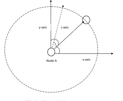
Angle of Arrival (AoA)

As in fig-3, node A transmits RF signal in Omni-directional pattern. Other node B in the line of sight of sender node and within communication range of A measures the bearing of this wave w.r.t some reference line or plane.

Different AoA measurement techniques exist as of now. In one method, array of RF antennas or microphones at receiver node help determining AoA. In these methods, several spatially separated microphones detect single transmitted signal. By analyzing the phase or time difference between the signal‟s arrival at different antennas or microphones, it is possible to discover the angle of arrival of the signal. In second method it is also possible to gather AoA data from optical communication methods. Using digital signal processing as in MUltiple Signal Identification and Classification (MUSIC) algorithm [11], the accuracy up to 10 of AoA estimation can be achieved. A comparison of all measurement techniques is given in table-2.

Type of measurement and its method depend upon type of application and architecture of WSN node. For example, for outdoor localization and tracking of animals, accuracy in cm is not that important as lifetime of nodes. Therefore RSSI or hop count based distance measurement is most suitable as low computational overhead will result into conservation of energy source and hence increased lifetime.

Fig-3: 3D AoA Measurement

Node A x-axis

Table 1. Comparison of TDoA methods

Method Extra Hardware requirement Synchronization between

nodes Effect of speed of sound

RF-RF No as RF Transceiver is already present in every node

Required at receiving nodes (effect of small synchronization error is

large).

No

RF-Ultrasonic

Yes as speaker microphone at ultrasonic frequency are generally not a part of sensor

node

Not required

Yes as speed of sound changes with temperature

and medium.

Ultrasonic - Ultrasonic

Yes as speaker microphone at ultrasonic frequency are generally not a part of sensor

node

Required at receiving nodes(effect of small synchronization error is

small)

No as both signals will undergo same change.

Table 2. Comparison of Measurement techniques.

Measurement Type Line of Sight

Accuracy

Non Line of Sight accuracy

Hardware Overhead

Computational Overhead

Distance

RSSI Less Very Low Low Low

ToA High High Low Low

TDoA Very High High High Low

Hop Count Low* Very low Low Low*

TWR High Very Low Low Low

Angle AoA High Very Low High Low

* For high accuracy complex computations are required

Whereas for an indoor scenario where energy source can be replaced periodically and accuracy is a concern, then TDoA based distance method, AoA or combination of two can be used.

6.

LIMITING FACTORS FOR WSN

LOCALIZATION

Due to their small size and the type of applications that are thought of sensor networks, the limiting factors which affect the throughput of localization are low cost, limited processing power and limited battery life. Majority of WSN platforms at present in use like TelosB/Tmote sky, MicaZ/Mica2, IRIS etc, have limited bus width from 8 to 16 bits, processor clock frequency from 4 to 8 MHz, memory in terms of few kilobytes, and are powered by two AA size batteries [12]. Only few of these platform support floating point arithmetic. With these specifications, expecting a node to perform a heavy duty complex artificial intelligence based localization algorithm is impractical. The core function of a WSN is to detect and report events. These events can be added with location information to make it meaningful using some data aggregation and routing algorithm. For most of the applications localization is done only once and sensing and routing many times over the lifetime of a node. A complex algorithm would take more time getting executed because of the lower CPU capabilities and also the energy source gets depleted. Reduced battery life eventually decreases the operating lifetime of a node. Similarly a lengthy algorithm

would take more space in the memory leaving small place for sensing, routing and other core operations. The need for low complex, small and energy efficient algorithm can be imagined from this.

7.

LOCALIZATION ALGORITHMS

More than 50 localization algorithms for localization in WSN exist till date. To discuss all of these algorithms is impractical; therefore we‟ll first broadly classify these algorithms into different categories and then discuss few most popular and realistic of them one by one. These algorithms can broadly be classified below.

7.1

Anchor based

7.2

Anchor Free

Anchor free algorithms also exist to date [16], [17]. But these algorithms provide a relative non unique map of the nodes in a WSN which can be used in limited applications like efficient routing.

7.3

Centralized Algorithms

In centralized algorithms, the computation task is done on a base station and this base station need not to be a WSN node; instead a more powerful system. This allows the centralized algorithms to be lengthy and complex. However the measurements from each node are required to be communicated to the base station. Range base localization algorithms depend upon the measurements like distance (through RSSI, ToA or TDoA) or angle to determine the location of an unknown node. Range based localization algorithm in its simplest form uses distance information from nodes neighboring anchor nodes and using trilateration determine its location.

Several complex algorithms like non linear least square approximation [18] reduce this error in localization. Other region based semi definite programming (SDP) takes all measurements viz a viz inter-node distance or angle or both measurements and creates probable regions of the unknown nodes. These Types of algorithms are up to 𝑂 𝑘3 _{complex in}

two dimensional scenarios. Second type of centralized localization algorithm (MDS-MAP) uses matrix of inter-node distance to create a local map of the system with 𝑂 𝑛3 _{complex operations. The local map thus creates can be}

stitched to the global map using anchor nodes [4]. Three dimensional localization using these techniques have not been implemented and can serve as a path for future research.

Another localization algorithm in [19] use distance measurement from TDoA and then statistical signal processing technique (Kalman filtering) to localize WSN node. This type of algorithm has not been verified experimentally; however the simulation results show accuracy

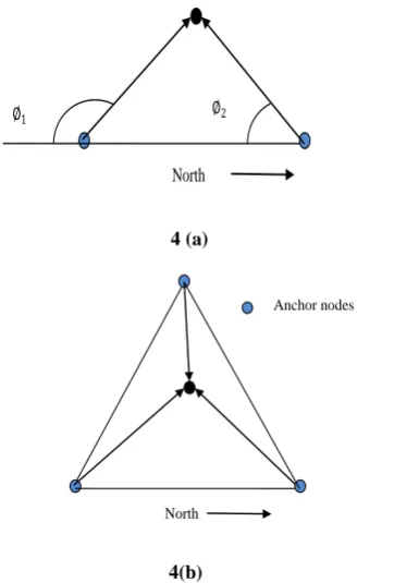
near to the Cramer Rao Bound. The complexity of the algorithm makes it fall into centralized algorithms‟ category. The simulation or implementation of trilateration or MDS-MAP using two way ranging can give promising results. Using AoA information and triangulation as shown in figure-5 below, location of an unknown node can be determined using at least two anchors in 2D [20] and three anchors in 3D scenario as shown in fig-4.

7.4

Distributed and Range Free

Algorithms

The advancements in the field of processor technology has made it possible to incorporate nodes that can compute algorithms for localization with high accuracy. In distributed approach the nodes communicate and cooperate with each other in determining their positions. The energy required to perform calculation on a data is much less than energy required in transmitting it to a base station far away. The situation is worst when a node is more than five hops away from base station. Range free algorithms do not depend upon any inter-node measurement, instead they use connectivity information or some limited form of RSSI for localization. These distributed algorithms can be range based or range free. Few of the popular distributed localization algorithms are given below.

7.4.1

Centroid Localization

In [21], authors propose an algorithm which is range free and distributed. Every node in the neighbor of other three or more anchor nodes approximates its position at the centroid of these nodes.

This updated position of a node helps localize other nodes in the neighborhood. The main advantage of this algorithm is its simplicity and no need for distance measurement. But the algorithm is not very accurate. In three dimensional spaces,

5(a)

5(b)

Fig-5. (a) 2D and (b) 3 D Centroid localization (𝑥3, 𝑦3)

(𝑥1, 𝑦1)

(𝑥2, 𝑦2)

(𝑥, 𝑦)

Anchor nodes

(𝑥3, 𝑦3, 𝑧3)

(𝑥1, 𝑦1, 𝑧1) (𝑥2, 𝑦2, 𝑧2)

(𝑥, 𝑦, 𝑧) (𝑥4, 𝑦4, 𝑧4)

4 (a)

4(b)

Fig-4. Triangulation in (a) 2D and (b) 3D North

∅2

∅1

Anchor nodes

four anchors would be required to form a tetrahedron and the node can be approximated to be at the centre of this tetrahedron as shown below in fig-5.

To increase its accuracy different modifications to this algorithm were done by different authors. Authors in [22] use same algorithm with small modification and achieve higher accuracy even in three dimensional space. An adaptive weights weighted centroid localization algorithm in [23], does not calculate simple average of anchor node points, but applies weights to anchor nodes depending upon their RSSI value. This further reduces the error of localization.

To improve the localization accuracy, a local gradient based refinement process can be added in the localization algorithm [24]. This type of algorithm is a hybrid exploiting advantages of both centralized and distributed algorithms.

7.4.2

Approximate point in triangle (APIT)

As explained in [4],authors in [25] propose an algorithm in which an unknown node determines whether it is inside a triangle formed by three anchors in the neighborhood or not. This decision is taken by reading RSSI values coming from anchor nodes. If it is inside the triangle of three anchors, the node‟s position is estimated to be centre of the triangle. Since this method does not use distance measurement and depend upon crude RSSI measurement, therefore there are sometimes errors in deciding whether an unknown node is inside the triangle or not, especially when it is near the edge of a triangle formed by anchors. The modified version of APIT in [26] overcomes this error by calculating individual areas of the triangles formed in both in-case and out-case and then comparing it with total area. This algorithm falls in the category of range free methods as RSSI in its crude form is used instead of refined distance value estimated from this RSSI. APIT has slightly larger communication overhead than Centroid but is more accurate than simple centroid method. More the number of anchor nodes, more are the triangles formed around unknown node and hence more accuracy as shown in fig-6 below.

Authors in [27] propose a three-dimensional localization algorithm (APIT-3D) based on APIT. It determines if an unknown node is in a tetrahedron which has four anchors and then, it takes the centroid of the tetrahedron as the estimated position of the unknown node.

7.4.3

Bounding Box

Another range free distributed localization algorithm is bounding box. In [24], authors proposed an algorithm where anchors form a square box around them with edges equal to twice the maximum range of an anchor as shown in fig-7(a) below.

This basic figure is formed around all the nearby anchors and any node within the communication range of these squares form a bonding box after intersection of all squares. The unknown node assumes its location to be at the centre of this box and this unknown can update itself as anchor and help other nodes localize themselves. The bounding box algorithm is simpler than centroid and APIT. But its accuracy is also less than these two algorithms. Moreover this algorithm has not been implemented or proposed for three dimensional scenarios. We present a three dimensional version of the same where instead of squares, the basic figure is a cube and the intersection of these cubes is also a three dimension polygon as shown in fig-7(b). To achieve accuracy sufficient for indoor localization, this scheme would need large number of anchor nodes.

Another distributed and range free algorithm [28] introduces localization using Self-Organizing Maps. By introducing the utilization of intersection areas between radio coverage of neighboring nodes, their algorithm maximizes the correlation between neighboring nodes in distributed SOM implementation. With this correlation maximization, their method increases the quality of the topology estimation and reduces the time of the convergence and the accuracy achieved is near to 30% of the maximum range. However the algorithm tends to be complex and it‟s the real implementation on 3D scenario is yet to be done.

7.5

Distributed and Range Based

In [29], authors assume that due to many factors there is noise in distance measurement using cheap RSSI. Therefore the help of probability theory is taken to reduce its effect on localization accuracy and a region based algorithm is proposed. Based on limited error in distance measurement a

7(a)

7(b)

Fig-7. (a) 2D and (b) 3 D Bounding Box localization Anchor nodes

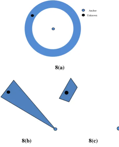
physical constraint with minimum and maximum distance is formed by each anchor on an unknown node. In this algorithm all unknown nodes initialize their region equal to the size of deployment area. Then two anchors help an unknown form its own constraint and thus feasibility region. The confidence with which a node can be said to be in the feasibility region formed depends upon the standard deviation in distance measurement. This feasibility region formed can further be reduced by adding confidence in form of new mean and standard deviation from another anchor in same hop or some other hop. As described in [30], more the distance in number of hops between anchor and unknown node, larger is the probability or feasibility region as a result of error propagation. The constraints formed by one anchor for an unknown node in distance, AoA only and the distance and AoA combine are shown in fig-8.

Authors in [30] propose probabilistic region based AoA based localization approach similar to [29]. The difference lies in the measurement that is AoA instead of distance using RSSI. This AoA based distributed localization algorithm achieves good accuracy and precision similar to [29]. But this algorithm still requires good percentage of anchors to achieve good accuracy.

Authors in [30] achieve sub meter accuracy in a deployment region of 100m x 100 m using AoA and maximum range information with single anchor and 100 unknowns. In [30] information is collaboratively used by the nodes from first hop to second and subsequent hops to reduce the error propagation and back tracing further increases accuracy and precision.

Some authors also propose a combination of distance and AoA measurement for localization [31] and [32]. Initial estimate of probability region using this approx is more accurate and error propagation is reduced in a better way. Authors in this paper propose to use these constraints in three dimensions to localize a WSN in three dimensions. The basic constraints formed in three dimensions using AoA and distance + AoA are shown in the fig-9.

Based on these constraints a collaborative multihop error reducing technique is expected to yield promising results.

7.6

Non Secure localization

All the localization schemes discussed above assume that deployment of WSN is in a trusted zone, where nodes have no security issues and there are no attacks of any kind on the network. Therefore these schemes can be placed altogether in non secure localization as these schemes are vulnerable to various attacks discussed below.

7.7

Secure localization

However in some applications like security surveillance, battlefield deployment, there may be different types of attacks on localization process itself as compromising localization or attacking localization to report wrong positions of nodes would make data useless. The localization process can be attacked at any stage of localization. Different type of attacks on localization and their proposed solutions till date are given below.

7.7.1

Range or Angle Attack

In this type of attack, in case of RSSI based distance estimation process, a compromised node in transmission mode may change the transmitted power from a fixed reference power making receiving node estimate wrong distance resulting into incorrect positions of nodes. In TDoA, the compromised transmitter node can change the fixed delay between two waves resulting into incorrect distance estimation. In AoA, the attacked transmitter node can stop transmission from reference (anchor) nodes and the receiving node would never know that an anchor is in the communication range. If a receiving node is compromised, the node can miscalculate distance or angle parameters.

7.7.2

Repudiation Attack

In repudiation attack, the transmitted node doesn‟t send its correct id to the transmitter. This attack would effect transmitter as well as receiver node. If a transmitter is compromised with this attack, the transmitting node send the data packet with RSSI/ TDoA or AoA information and will and appear to be some other node. This will make ranging process near to impossible for a receiver. If receiver is compromised, the data log of receiver pertaining to localization cannot be relied upon.

7.7.3

Wormhole attack

In this attack, the compromised nodes communicate with each other while recording their wrong positions, resulting into incorrect localization.

9(a) 9(b)

Fig-9. 3D Constraints using (a) AoA only and (b) Distance + AoA

Anchor Unknown

8(a)

8(b) 8(c)

Fig-8. 2D Constraints in (a) distance only, (b) AoA only and (c) combined

7.7.4

Forging/Replay

Easiest of all attacks, this type of attack can be executed even by the nodes with limited recourses as the attacking node doesn‟t have to do any complex processing for attack. This type of attack can be explained well with the help of an example. For example a node A transmits a data packet including its ID to node B. An attacking node C in the communication range of both A and B can also receive this packet. Now C has to simply retransmit this packet to B in its original format. It will become difficult for B to recognize whether A or C node is sending legitimate packet. A more sophisticated form of this attack is called Sybil attack in which an attacking node takes the identity of several nodes including anchor nodes affecting localization process in a big way.

7.8

Security measures

In [33] authors use four inherent properties of WSN to detect attack. These four properties are used for ranging attack and include the temporal property of the locators, the spatial property of the locators, the consistent property of the legitimate locators, and the consistent property of the attacked locators. Under temporal property of the locators, the detection of attack is done if the sensor receives more than one signal from a locator. Under spatial property of the locators, if sensor node receives messages from two different locators for each localization procedure and the distance between these two locators are larger than twice of maximum range of a node, this means one of these two locators is attacked. The consistent property of legitimate locators and attacked locators is similar to as in [34]. However in practical world, a WSN attacked by Sybil or wormhole attack can change or reverse the scenario where most of the nodes may be compromised sending wrong data. Therefore there is need to prevent the attack firsthand or at least make reduce the effect of localization at the initial stage of measurements and observations.

Authors in [35] and [36] propose a trilateration based technique for position verification called Verifiable Multilateration (VM), which relies on distance bounds. In VM, if a node is inside the triangle formed by three nodes with known locations, and distance is within the maximum bounds, node‟s location can be uniquely determined. In other method, SPINE introduced by the same authors, all the distance measurements are verified by VM triangles around them formed by sensor nodes, preventing nodes to produce erroneous distance measurements. In [37] authors propose the use of some special and powerful locator nodes which are capable of steering their RF beam and the unknown nodes in the network can determine their position at the centre of intersections of the constraints formed by the messages received from several locators. As this method does not depend upon any distance or angle measurement, therefore ranging attacks do not apply to this type of localization technique. In [34] authors propose two methods for secure localization. In first method, using attack-resistant Minimum Mean Square Estimation (MMSE), the compromised anchor nodes‟ data packets are filtered out by identifying the inconsistency in them, indicated by MMSE. In second method, authors introduce location reference “vote” on the locations at which the node of concern may reside. To facilitate the voting process, the target field is quantized into a grid of cells, where each sensor node determines how likely it is in each cell based on each location reference. Cell(s) with the highest vote are then selected and center of the cell(s) are treated as estimated location(s). These schemes also assume

that security key management also exists for identification of anchor nodes.

8.

CONCLUSION AND FUTURE WORK

Localization in wireless sensor networks is an important issue. Considering the hardware and cost limitations of a node, energy efficiency, computational cost, accuracy and security are the metrics for the performance of any localization scheme. Selection of measurement type depends upon the type of application and deployment scenario. For three dimensional scenarios, computation and communication increases drastically, compared to two dimension localization. While RSSI some limitations, in terms of providing less accurate initial estimate for distance, still it has been favored by researchers, because of its low cost compared to any other measurement technique, especially for 3D localization. Some of the algorithms have high energy efficiency with low computational cost but their application in high accuracy requirement scenario is impractical. These types of schemes are applicable for localization of WSN used outdoors .Indoor applications demand high accuracy. Authors in this paper have also proposed a direction in 3D localization using regional constraints in 3D spaces. Making localization process more accurate needs more resources making it less energy and computational efficient. Security is required for some non civil applications but it adds to the energy cost. In short, generally for a localization approach the trade offs in localization metrics exists, but for a specific application, these tradeoffs may not play an important role.

9.

REFERENCES

[1] A. Srinivasan And J. Wu, “A Survey On Secure Localization In Wireless Sensor Networks,” Encyclopedia Of Wireless And Mobile Communications, B. Furht (Ed.), CRC Press, Taylor And Francis Group, 2008.

[2] Ammar, W., Eldawy, A., And Youssef, M. “Secure Localization In Wireless Sensor Networks: A Survey”. In Proceedings Of Corr. 2010.

[3] Zhetao Li, Renfa Li, Yehua Wei And Tingrui Pei, “Survey Of Localization Techniques In Wireless Sensor Networks.” Information Technology Journal. 9(2010): 1754-1757.

[4] J. Bachrach And C. Taylor. “Localization In Sensor Networks”. Handbook Of Sensor Networks: Algorithms And Architectures, 1st Ed., 1, 2005.

[5] Mourad, F., Snoussi, H., Abdallah, F., Richard, C., “Anchor-Based Localization Via Interval Analysis For Mobile Ad-Hoc Sensor Networks,” Signal Processing, IEEE Transactions On , Vol.57, No.8, Pp.3226-3239, Aug. 2009.

[6] J. Seybold, “Introduction to RF Propagation”, Wiley Interscience, 2005.

[7] K. Benkic, M. Malajner, P. Planinsic, And Z. Cucej, “Using RSSI Value For Distance Estimation In Wireless Sensor Networks Based On Zigbee,” In Proceedings Of The 15th Conference On Systems, Signals And Image Processing, Pp. 303–306, 2008.

[9] Weile Zhang, Qinye Yin, Xue Feng; Wenjie Wang, “Distributed TDOA Estimation For Wireless Sensor Networks Based On Frequency-Hopping In Multipath Environment,” Vehicular Technology Conference (VTC 2010-Spring), 2010 IEEE 71st , Vol., No., Pp.1-5, 16-19 May 2010.

[10]H. Balakrishnan, R. Baliga, D. Curtis, M. Goraczko, A. Miu, N. Priyantha, A. Smith, K. Steele, S. Teller, And K. Wang. “Lessons from Developing And Deploying The Cricket Indoor Location System. Preprint.” November 2003.

[11]Klukas, R., Fattouche, M., “Line-Of-Sight Angle Of Arrival Estimation In The Outdoor Multipath Environment,” Vehicular Technology, IEEE Transactions On , Vol.47, No.1, Pp.342-351, Feb 1998. [12]M. Johnson, P. Van De Ven, M.Healy, And M.J. Hayes,

“A Comparative Review Of Wireless Sensor Network Mote Technologies”, Proc. IEEE Sensors Conference, Pp 1695-1701, Auckland, New Zealand, November, 2009. [13]Jang-Ping Sheu, Pei-Chun Chen, Chih-Shun Hsu, “A

Distributed Localization Scheme For Wireless Sensor Networks With Improved Grid-Scan And Vector-Based Refinement,” Mobile Computing, IEEE Transactions On , Vol.7, No.9, Pp.1110-1123, Sept. 2008.

[14]Yu, K., Sharp, I. And Guo, Y. J., “Anchor-Based Localization For Wireless Sensor Networks, In Ground-Based Wireless Positioning”, John Wiley & Sons, Ltd, Chichester, UK, 2009.

[15]Bin Xiao, Lin Chen, Qingjun Xiao, Minglu Li, , "Reliable Anchor-Based Sensor Localization In Irregular Areas," Mobile Computing, IEEE Transactions On , Vol.9, No.1, Pp.60-72, Jan. 2010.

[16]Priyantha, N. B., Balakrishnan, H., Demaine, E., & Teller, S. “Anchor-Free Distributed Localization In Sensor Networks” (Tech. Rep. No. 892). MIT Laboratory For Computer Science, 2003.

[17]Fang, L., Du, W., & Ning, P., “A Beacon-Less Location Discovery Scheme For Wireless Sensor Networks”. In Proceedings Of Annual Joint Conference Of The IEEE Computer And Communications Societies (Pp. 161– 171), 2005.

[18]Samir S. Sahyoun, Seddik M. Djouadi, Hairong Qi, And Anis Drira, “Source Localization Using Stochastic Approximation And Least Squares Methods.” 2nd Mediterranean Conference On Intelligent Systems And Automation (Cisa'09). AIP Conference Proceedings, Volume 1107, Pp. 59-64, 2009.

[19]Chen Hongyang, Deng Ping, Xu Yongjun, And Li Xiaowei, "A Robust Location Algorithm With Biased Extended Kalman Filtering Of TDOA Data For Wireless Sensor Networks," IEEE Comput, Pp.883-886, 2005. [20]D. Nicolescu And B. Nath, “Ad-Hoc Positioning

Systems (APS),” In Proceedings Of IEEE GLOBECOM „01, November, 2001.

[21]N. Bulusu, J. Heidemann And D. Estrin, “GPS-Less Low Cost Outdoor Localization For Very Small Devices,” IEEE Personal Communication Magazine, Newblock Vol. 7, No. 5, October 2000, Pp. 28-34.

[22]Hongyang Chen, Pei Huang, Marcelo Martins And Kaoru Sezaki, “Novel Centroid Localization Algorithm For Three-Dimensional Wireless Sensor Networks,” In

Pro. IEEE Wicom '08. 4th International Conference On Oct, 2008, Pp. 1-4.

[23]Ximei Liu, Chao Zhang, Jizhen Hu, , “Adaptive Weights Weighted Centroid Localization Algorithm For Wireless Sensor Networks,” Wireless Communications, Networking And Mobile Computing, 2008. 4th International Conference On , Vol., No., Pp.1-4, 12-14 Oct, 2008.

[24]T.C. Liang, T.C. Wang, And Y. Ye. “A Gradient Search Method To Round The Semidefinite Programming Relaxation Solution For Ad Hoc Wireless Sensor Network Localization.” In Tech. Rep., Dept Of Management Science And Engineering, Stanford University, 2004.

[25]He T, Huang CD, Blum BM, Stankovic JA, Abdelzaher T. “Range-Free Localization Schemes In Large Scale Sensor Networks.” In: Proc. Of The 9th Annual Int‟l Conf. On Mobile Computing And Networking. San Diego: ACM Press, 2003.

[26]Ji Zeng Wang, Hongxu Jin, “Improvement On APIT Localization Algorithms For Wireless Sensor Networks,” Networks Security, Wireless Communications And Trusted Computing, 2009. International Conference On , Vol.1, No., Pp.719-723, 25-26 April 2009.

[27]Liu Yuheng, Pu Junhua, He Yang etc. “Three-dimensional self-localization scheme for wireless sensor networks”, Journal of Beijing University of Aeronautics and Astronautics. 2008. 34(6): 647~651.

[28]P. D. Tinh And M. Kawai, “Distributed Range-Free Localization Algorithm Based On Self-Organizing Maps,” EURASIP Journal On Wireless Communications And Networking, Vol. 2010, 2010.

[29]V. Ramadurai And M.L. Sichitiu, “Localization In Wireless Sensor Networks: A Probabilistic Approach”, In Proc. International Conference On Wireless Networks, 2003, Pp.275-281.

[30]S.B. Kotwal, S. Verma, Suryansh, Arnav Sharma, G.S.Tomar, “Region Based Collaborative Angle Of Arrival Localization For Wireless Sensor Networks With Maximum Range Information,” CICN, International Conference On, Pp. 301-307, 2010.

[31]Chulyoung Park, Daeheon Park, Jangwoo Park, Yangsun Lee, Youngeun An, , “Localization Algorithm Design And Implementation To Utilization RSSI And AOA Of Zigbee," Future Information Technology (Futuretech), 2010 5th International Conference On , Vol., No., Pp.1-4, 21-23 May 2010.

[32]S.B. Kotwal, Shekhar Verma, G.S. Tomar, R.K. Abrol, “MAIL: Multi-Hop Adaptive Iterative Localization For Wireless Sensor Networks,” Cicsyn, Pp.149-154, 2009 First International Conference On Computational Intelligence, Communication Systems And Networks, 2009.

[33]Honglong Chen, Wei Lou, And Zhi Wang, “A Novel Secure Localization Approach In Wireless Sensor Networks,” EURASIP Journal On Wireless Communications And Networking, Vol. 2010, Article ID 981280, 12 Pages, 2010.

Processing In Sensor Networks (IPSN ‟05), Pages 99-106, April 2005.

[35]S. Capkun and J.-P. Hubaux, “Secure positioning of wireless devices with application to sensor networks,” in Proceedings of INFOCOM, 2005.

[36]S. Capkun and J. P. Hubaux, “Secure positioning in wireless networks”, IEEE J. Sel. Areas Commun., 2006. [37]Lazos, L., Poovendran, R., , “HiRLoc: high-resolution