A test of the normality assumption in the ordered probit model

(1)

Munich Personal RePEc Archive

A test of the normality assumption in

the ordered probit model

Johnson, Paul A.

Vassar College

1996

Online at

https://mpra.ub.uni-muenchen.de/10080/

(2)

Published as "A Test of the Normality Assumption in the Ordered Probit Model," 1996, METRON, LIV:213-21.

A Test of the Normality Assumption

in the Ordered Probit Model

Paul A. Johnson Department of Economics

Vassar College Poughkeepsie, NY 12601

USA

December, 1995

This paper presents an easily implemented test of the assumption of a normally distributed error term for the ordered probit model. As this assumption is the central maintained hypothesis in all estimation and testing based on this model, the test ought to serve as a key specification test in applied research. A small Monte Carlo experiment suggests that the test has good size and power properties.

Key words: Order Probit, Normality, Lagrange Multiplier

(3)

1 1. Introduction

Despite the growing number of applications, the literature does not include a test of the normality assumption for the ordered probit model. As Bera, Jarque and Lee (1984), hereafter BJL, point out, the validity of the normality assumption is more important in limited dependent variables models than in the usual regression model as, if the assumption does not hold, maximum likelihood estimation will not, in general, yield consistent parameter estimates. The assumption is also the central maintained hypothesis in any statistical inference based on the parameter estimates. In addition, normality of the error term is crucial to the interpretation of the effects of changes in the explanatory variables as these effects are usually expressed in terms of changes in the probabilities of each of the outcomes.1

In this paper I extend the work of BJL and derive a Lagrange multiplier, hereafter LM, test of the normality assumption for the ordered probit model. The test is easily implemented and should also serve as a general specification test of the ordered probit model. I examine the properties of the test in a small Monte Carlo experiment and find that, while the actual size of the test may exceed its nominal size somewhat in small samples, the test has good power properties, at least against the class of alternatives considered.

2. A Test for Normality

Let be the dependent variable of interest and assume _  _   where is a –vector of 

  

 

exogenous variables is a –vector of parameters, and is a zero-mean error term, distributed   

identically and independently across with distribution function       having parameters . Rather

than observe , all that is known is which of intervals, forming a partition of the real line, contains 



            

 Define      and let

      

   



 if _otherwise 

1_{For a graphical exposition of the ordered probit model see Becker and Kennedy (1992) who also discuss the pitfalls and}

(4)

for      . It follows that                      The log likelihood for a sample of observations is

                      

      

          

The parameters       and may be estimated consistently by the maximizers of this

function under suitable regularity conditions.2

When is the standard normal distribution, , the model outlined above is the ordered probit 

model. In this note I develop a test of the hypothesis that is the standard normal distribution against

the alternative that it is some other member of the Pearson family of distributions. The Pearson family has distribution functions which can be written as             where

 _       

   

and  (see BJL or Johnson and Kotz (1970) for details). When

   

   and        , is the standard normal distribution. Because    is the normalization

imposed to identify the parameters of the ordered probit model, the null hypothesis to be tested here is

      .

Defining   , the log likelihood under the alternative hypothesis is

                           

     

 

where . Evaluated at

the null values of       , after imposing the normalization    , the derivatives of with

respect to the parameters are

(5)

3                             _{  }      _ _{   }   _                                

for ;

                    _{  }                  _{  }         ;

3 ; and,

,

1 

   



where ( ) is the standard normal density function and is a standard normal random variable.  

It can be shown that3

                                                                 

  ; and,

                                            

These results may be used to write

    _{  }       _{  } _{ } _{       }     _{  }  _{  } _ _ _                   

1  

 



3 ; and,

                          .

In order to compute the test statistic define

3_{The results in Johnson and Kotz (1970) p81-83 and the recursion}_ _ _for

 

 _  _ _ _

(6)

                                                                                              _{  }  _        _ _        where    _{  }   _                                                               

The LM test statistic for the hypothesis that is normally distributed may then be computed as

 _ _{ }   _ __                 

where is a matrix consisting of the last two columns of an       dimensional identity matrix and all of the elements of are evaluated at their ordered probit MLE values. The proofs in the appendix to

BJL may be modified to show that, under the null hypothesis, is asymptotically distributed as a  2

random variable with two degrees of freedom.

3. A Monte Carlo Experiment

To examine the properties of the test I conduct a small Monte Carlo experiment. The model is specified as    _ with distributed uniformly on     ,  ,   and  . I

    

      

 

perform 10000 replications for each of several distributions for having zero mean and unit variance

and each of the sample sizes 250, 500, 750, and 1000 To examine the size of the test is drawn from 

(7)

5

The gamma distribution is the member of the Pearson family generated by setting    with

   Here   _ so that the density of  under the alternatives is

      _{ }        __     

 _ _ _

  

   

 

for  . Note that, as , c so

  I use   and . Figure 1 plots these three density functions and 4 . As the figure

indicates,     becomes less skewed to the right as increases and for    it is quite close to



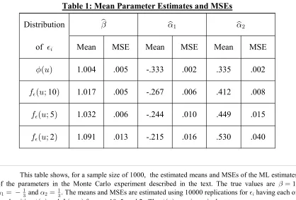
Tables 1 and 2 give the results of the Monte Carlo experiment. Table 1 shows the estimated means and MSEs of the parameter estimates for the sample size of 1000. The results for the other sample sizes are similar and not reported to save space. The first row shows that when the assumption

4_For__{  }_{and , was constructed as}_ __ ___{ }  _{  }_ __{with the drawn from a}__ _{  }_distribution_ 

 

(8)

of a normally distributed error is true the distributions of the ML estimates are centered on the respective true values of the parameters. The other three rows show that, as the deviation of the distribution of the error term from normality increases, as measured by the decline in (or, equivalently, the skewness of

the distribution) so does both the bias and MSE of the ML estimates. This is particularly so for and

 with the result that the gap between them increases with the skewness of the distribution of the error

[image:8.612.98.516.229.511.2]

term. Estimated outcome probabilities and their derivatives with respect to will be accordingly biased.

Table 1: Mean Parameter Estimates and MSEs Distribution

of Mean MSE Mean MSE Mean MSE

1.004 .005 -.333 .002 .335 .002

10 1.017 .005 -.267 .006 .412 .008

5 1.032 .006

  





 _ _



  

 





 -.244 .010 .449 .015

2 1.091 .013 -.215 .016 .530 .040

  

This table shows, for a sample size of 1000, the estimated means and MSEs of the ML estimates of the parameters in the Monte Carlo experiment described in the text. The true values are  ,

 _ and  _. The means and MSEs are estimated using 10000 replications for having each of

the densities  and     for 10, 5, and 2. The  case is equivalent to  .

Table 2 shows the percentage of rejections for a 5% test of the hypothesis that the error term is normally distributed for each of the sample sizes and each of the densities of the error term. When has

(9)

[image:9.612.134.477.57.271.2]

7

Table 2: Percentage of Rejections of Normality Hypothesis

Sample Density of

Size 10 5 2

250 6.6 16.2 28.1 79.4

500 5.3 24.4 48.8 97.7

750 5.1 34.4 66.5 99.8

1000 5.0 43.7 78.5 100.0







         

This table shows, for each of the indicated sample sizes, the percentage of rejections of the hypothesis that has a normal distribution using the test described in the text with an asymptotic

size of 5% for having the densities   and     for 10, 5, and 2. In the first case, which is equivalent to  , this percentage estimates the size of the test, while in the others, it indicates the power against that particular deviation from the null. In each case 10000 replications were performed.

Overall, conditional on the setup of the Monte Carlo experiment, the size and power properties of the test appear to be quite good. The size of the test may slightly exceed the nominal value in small samples but rapidly approaches 5% as the sample size rises. The power of the test increases with both the magnitude of the deviation from the null, as measured by the skewness of the distribution of the error term, and with the sample size. In the case of having the density     2 , which is the furthest from the null of normality, the power is never less than 79% and reaches 100% for the 1000 observation sample.

4. Conclusions

(10)

References

[1] Amemiya, Takeshi, (1985), Advanced Econometrics, Harvard University Press, Cambridge.

[2] Becker, William E., and Peter E. Kennedy, (1992), “A Graphical Exposition of the Ordered Probit,” Econometric Theory, 8:127–31.

[3] Bera, Anil K., Carlos M. Jarque and Lung-Fei Lee, (1984), “Testing the Normality Assumption in Limited Dependent Variable Models,” International Economic Review, 25:563–578.