An intercomparison and evaluation of aircraft derived and simulated CO from seven chemical transport models during the TRACE P experiment

(1)

An intercomparison and evaluation of aircraft-derived and simulated

CO from seven chemical transport models during the TRACE-P

experiment

Christopher M. Kiley,1Henry E. Fuelberg,1Paul I. Palmer,2 Dale J. Allen,3 Gregory R. Carmichael,4 Daniel J. Jacob,2,8 Celine Mari,5 R. Bradley Pierce,6 Kenneth E. Pickering,3Youhua Tang,4Oliver Wild,7 T. Duncan Fairlie,6,8 Jennifer A. Logan,8 Glen W. Sachse,6Todd K. Shaack,9 and David G. Streets10 Received 29 October 2002; revised 14 March 2003; accepted 26 March 2003; published 15 November 2003.

[1] Four global scale and three regional scale chemical transport models are

intercompared and evaluated during NASA’s Transport and Chemical Evolution over the Pacific (TRACE-P) experiment. Model simulated and measured CO are statistically analyzed along aircraft flight tracks. Results for the combination of 11 flights show an overall negative bias in simulated CO. Biases are most pronounced during large CO events. Statistical agreements vary greatly among the individual flights. Those flights with the greatest range of CO values tend to be the worst simulated. However, for each given flight, the models generally provide similar relative results. The models exhibit difficulties simulating intense CO plumes. CO error is found to be greatest in the lower troposphere. Convective mass flux is shown to be very important, particularly near emissions source regions. Occasionally meteorological lift associated with excessive model-calculated mass fluxes leads to an overestimation of middle and upper tropospheric mixing ratios. Planetary Boundary Layer (PBL) depth is found to play an important role in simulating intense CO plumes. PBL depth is shown to cap plumes, confining heavy pollution to the very lowest levels. INDEXTERMS:0341 Atmospheric Composition and Structure: Middle atmosphere—constituent transport and chemistry (3334); 0345 Atmospheric Composition and Structure: Pollution—urban and regional (0305); 0365 Atmospheric Composition and Structure:

Troposphere—composition and chemistry; 0368 Atmospheric Composition and Structure: Troposphere— constituent transport and chemistry

Citation: Kiley, C. M., et al., An intercomparison and evaluation of aircraft-derived and simulated CO from seven chemical transport

models during the TRACE-P experiment,J. Geophys. Res.,108(D21), 8819, doi:10.1029/2002JD003089, 2003.

1. Introduction

[2] NASA’s Transport and Chemical Evolution over the

Pacific (TRACE-P) experiment, conducted between Febru-ary and April 2001, sought to characterize the chemical composition of Asian outflow and describe its evolution over the Pacific Basin. The goals of TRACE-P were to improve our knowledge of the Asian sources of climatically important atmospheric species and to understand the impli-cations for global atmospheric budgets [Jacob et al., 2003]. In addition to in situ chemical measurements by two NASA aircraft (a DC-8 and P-3B), TRACE-P included a major support activity from several three-dimensional (3-D) chem-ical transport models (CTMs) that were used in real time to optimize flight strategies.

[3] Many evaluations of individual CTMs have been

conducted previously [e.g., Allen et al., 1996a, 1996b;

Bey et al., 2001; Wild and Prather, 2000]. However, very few intercomparisons of different CTMs appear in the literature.Jacob et al.[1997] performed a model intercom-parison of radon simulations, whileKanakidou et al.[1999] evaluated carbon monoxide as a tracer.Rasch et al.[2000]

1_{Department of Meteorology, Florida State University, Tallahassee,}

Florida, USA.

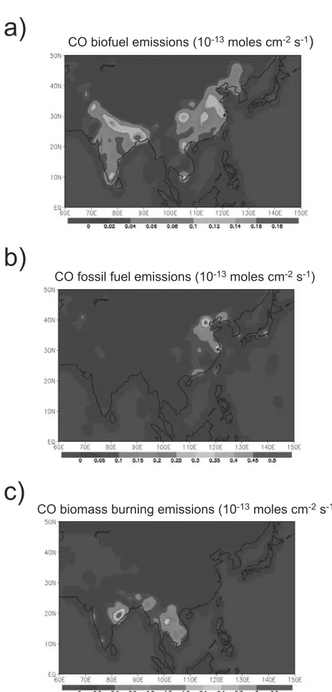
2_{Division of Engineering and Applied Sciences, Harvard University,}

Cambridge, Massachusetts, USA.

3_{Department of Meteorology, University of Maryland, College Park,}

Maryland, USA.

4_{Center for Global and Regional Environmental Research and}

Department of Chemical and Biochemical Engineering, University of Iowa, Iowa City, Iowa, USA.

5

Laboratorie d’Aerologie, UMR CNRS/Universite Paul Sabatier, Toulouse, France.

6_{NASA Langley Research Center, Hampton, Virginia, USA.} 7

Frontier Research System for Global Change, Yokohama, Japan.

8_{Department of Earth and Planetary Sciences, Harvard University,}

Cambridge, Massachusetts, USA.

9_{Space Science and Engineering Center, University of Wisconsin,}

Madison, Wisconsin, USA.

10

Argonne National Laboratory, Argonne, Illinois, USA.

(2)

compared simulations of radon, lead, sulfur dioxide, and sulfate, and Carmichael et al. [2002] evaluated the long-range transport of sulfur deposition. The large number of 3-D CTMs run during TRACE-P provides a unique opportunity to determine how the transport simulations compare among themselves and with observations. That was the goal of this research.

[4] Seven 3-D CTMs that were run during TRACE-P

participated in the intercomparison. They differ in several ways including domain size, resolution, meteorological fields, and their approaches and detail for simulating chem-ical processes and deposition.

[5] Carbon monoxide, a tracer common to all seven

models, was selected as the intercomparison species. Car-bon monoxide is a product of incomplete combustion and also is produced within the atmosphere by the oxidation of volatile organic compounds. The lifetime of carbon mon-oxide varies as a function of season and latitude but is on the order of months [Talbot et al., 1996]. Carbon monoxide has a relatively simple and well-understood chemistry and better documented, but still rather uncertain, direct sources than most shorter-lived species. Therefore it is a good species with which to evaluate the chemical and transport characteristics of tracer models [Kanakidou et al., 1999].

[6] The intercomparison has two major objectives. First,

we statistically analyze the aircraft-derived and seven numerically derived versions of CO. These CTM simula-tions were prepared following the field phase of TRACE-P using a common set of emissions. The resulting statistics document the overall ability of the CTMs to simulate CO. The analyses examine plumes of CO, focusing on their concentrations, as well as their horizontal placements, altitudes, and depths. Next, we identify and draw attention to the key meteorological processes that influence CTM performance. We focus on how differing parameterizations related to boundary layer processes and deep convection affect each model’s CO simulations. Our intent is to compare each model’s simulations with the others and with observations, looking for similarities and differences, and searching for possible explanations.

2. Data and Methodologies

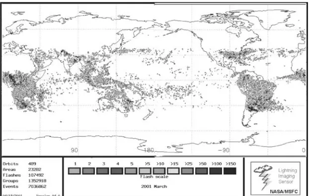
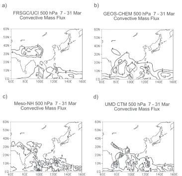
2.1. Chemical Transport Models

[7] Results from seven CTMs were examined in the

study, three regional models and four global models. Details of each model are shown in Table 1, and a brief description of each model is given below.

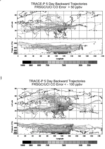
2.1.1. FRSGC//UCI

[8] The Frontier Research System for Global Change/

University of California, Irvine (FRSGC/UCI) global CTM [Wild and Prather, 2000] was run at T63 horizontal reso-lution (1.91.9) with 30 Eta levels in the vertical. For the current simulations it was driven by 3-hourly meteoro-logical fields generated by the European Centre for Medium Range Weather Forecasts (ECMWF) Integrated Forecast System [Wild et al., 2003]. Convective mass flux, cloud cover, precipitation and boundary layer height were sup-plied by the meteorological fields. Advection was calculated using the Prather scheme that conserves second-order moments [Prather, 1986]. Turbulent mixing was simulated by simple bulk mixing of the boundary layer at each model

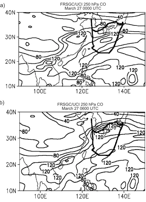
step. The model uses the ASAD package for gas-phase tropospheric chemistry [Carver et al., 1997], supplemented by a hydrocarbon oxidation scheme and a simplified treat-ment of stratospheric chemistry using the Linoz approach [McLinden et al., 2000].

2.1.2. GEOS-CHEM

[9] The Goddard Earth Observing System-Chemistry

model of tropospheric chemistry (GEOS-CHEM) global CTM [Bey et al., 2001;Martin et al., 2003] was run at a horizontal resolution of 2.02.5with 48 sigma levels in the vertical. It was driven by GEOS-3 assimilated mete-orological data from the NASA Data Assimilation Office. The 3-D meteorological data were updated every 6 hours, while mixing depths and surface fields were updated every 3 hours. Advection was calculated using a semi-Lagrangian scheme [Lin and Rood, 1996]. Moist convection was computed using GEOS data for convective, entrainment, and detrainment mass fluxes [Allen et al., 1996b]. In the current study, GEOS-CHEM was used in an offline chem-istry mode. Loss of CO was computed using archived monthly mean fields of OH concentrations from a full-chemistry simulation [Martin et al., 2003].

2.1.3. Meso-NH

[10] The Meso-NH regional nonhydrostatic mesoscale

meteorological model [Lafore et al., 1998; Mari et al., 1999; Suhre et al., 2000; Tulet et al., 2003] was run at a horizontal resolution of 75 75 km with 72 pressure levels in the vertical. The vertical resolution was 50 m in the boundary layer and 400 m above the boundary layer up to 20 km. Boundary layer height was calculated as the altitude of the near surface layer having turbulent kinetic energy greater than 0.25 m2 s 2. The boundary layer height was restricted to the first 3500 m to avoid turbu-lence from clouds. The domain was 0.76– 59.3N and 59– 180E. The dynamical time step was 60 s. Large-scale forcing of dynamical parameters was provided by ECMWF analyses at 6 hourly intervals. Convective mass flux was calculated within a convective mass transport algorithm. A CO tracer was introduced into the model to simulate the long-range transport of pollution. The tracer had the same primary source as carbon monoxide but had no indirect sources from the oxidation of methane or non-methane hydrocarbons. This tracer was coupled online with the model’s transport (advection, convection, turbu-lent mixing). Initial and boundary conditions of CO were provided by GEOS-CHEM at six hourly intervals. [Bey et al., 2001].

2.1.4. RAQMS-Global

[11] The Regional Air Quality Modeling System

(3)

T able 1 . Descriptions of the Seven CTMs That W ere Investigated in the S tudy FRSGC /UCI GEO S-CHEM v4.2 0 RAQM S-G lobal U M D CTM Meso-NH v4.3.1 RAQM S-Region al STEM v. Y2K1 Institutions: Fr

ontier Research System

(4)

climate simulation used the TRACE-P CO emission data set. Meteorological forecasts were reinitialized every 6 hours using ECMWF analysis. Convective mass flux, cloud cover, precipitation, and boundary layer height were supplied by the meteorological fields. The RAQMS-Global chemical predic-tions spanned the entire TRACE-P period. Advection was calculated using a flux form piecewise parabolic method. RAQMS includes standard stratospheric Ox-ClOx-BrOx-HOx-NOx cycles and oxidation of CH4and CO to account

for background tropospheric ozone production.

2.1.5. RAQMS-Regional

[12] The Regional Air Quality Modeling System

(RAQMS) regional meteorological and chemical model was run at a horizontal resolution of 110 110 km, with 50 vertical levels. The domain was 2– 48N and 76– 154E, and the dynamical time step was 2 min. Calculations were conducted online using instantaneous meteorological conditions from the UW Non-hydrostatic Modeling System (UW-NMS) [Tripoli, 1997]. ECMWF analyses were used for meteorological boundary conditions and to initialize the UW-NMS. Advection was calculated using a 6th order Crowler scheme in flux form. The RAQMS chemical module was the IMPACT model described above [Pierce et al., 2000; Al-Saadi et al., 2001]. Initial and boundary conditions of CO were provided by RAQMS-Global at six hourly intervals.

2.1.6. STEM

[13] The Sulfur Transport Eulerian Model (STEM)

regional CTM [Carmichael et al., 1986, 1990] was run at a horizontal resolution of 80 80 km, with 18 vertical levels defined in the Regional Atmospheric Modeling System’s (RAMS) sigma-z coordinate system. The domain was 8– 53N and 75– 163E, and the dynamical time step was 10 min. Large-scale forcing of dynamical param-eters was provided by RAMS driven by 6 hourly ECMWF reanalysis data. Advection was calculated using the Galerkin scheme [McRae et al., 1982]. Convective mass flux, cloud cover, precipitation, and boundary layer height were sup-plied by the meteorological fields, while convective and vertical diffusion were computed using a simple K scheme. STEM employs a chemical mechanism tool, the kinetic preprocessor for chemical mechanism (KPP), to determine the chemical reactions. For the current simulations STEM used the SAPRC99 chemical mechanism [Carter, 2000] and the second-order Rosenbrock method [Verwer et al., 1999]. Initial and boundary conditions of CO were specified by fixed vertical profiles. The lateral boundary condition (LBC) was based on TRACE-P P3-B Flight 11 which flew over the South China Sea. This flight’s CO profile was thought to best represent background values over water. The LBC varied vertically, but not horizontally. The LBC over land was obtained by adding 40 ppbv to the CO profile over water. This technique is based on experimental results. India and Russia are the primary inflow LBC for southern and northern portions of the TRACE-P domain, respectively. Characteristics of Indian outflow are described byDe Gouw et al. [2001]. For the northern LBC, only measurements from surface stations were available.Pochanart et al.[2003] discuss the Siberian airmass and European inflow.

2.1.7. UMD CTM

[14] A stretched-grid version of The University of

Mary-land Chemistry and Transport Model (UMD CTM) [Allen et

al., 2000] was run on a horizontal grid with 0.5 0.5 resolution in the region of interest (10– 40N; 100– 150E), stretching to 2.2(in longitude)1.9(in latitude) on the opposite side of the globe, with 17 sigma and 18 pressure levels in the vertical. The model was driven by 6 hourly meteorological fields from version 3 of the Goddard Earth Observing System Stretched-Grid Data Assimilation System (GEOS-3 SG-DAS) [Fox-Rabinovitz et al., 2002]. Planetary boundary layer depth, upward cloud mass flux and detrainment were supplied by the meteorological fields. Advection was calculated using a nonuniform grid version [Allen et al., 2000] ofLin and Rood’s [1996] multidimen-sional and semi-Lagrangian extension of the piecewise parabolic method [Colella and Woodward, 1984]. Vertical transport of trace gases by deep convection was parameter-ized using cumulus mass flux and detrainment profiles from GEOS-3 SG-DAS [Allen et al., 1996b]. Since convection in the GEOS-3 SG-DAS is performed on a uniform 11grid, these fields were interpolated onto the stretched-grid before use. Turbulent mixing was calculated through a fractional mixing scheme [Allen et al., 1996a] in which complete mixing of the boundary layer is assumed. Chemical produc-tion and loss of CO were prescribed in a manner similar to that ofAllen et al.[1996b] (i.e., prescribed OH concentra-tions [Spivakovsky et al., 2000] are used for computing CO loss and CO production from CH4). Carbon monoxide yields

from oxidation of nonmethane hydrocarbons were prescribed as in the work ofAllen et al.[1996b].

2.2. Emissions Data

[15] The special simulations reported here were prepared

after the field phase of TRACE-P was completed, i.e., they are not the simulations used during real time flight planning. Five of the seven CTMs used the same initial CO distribu-tions on the first date of their TRACE-P simulation, 15 February 2001. This common initial CO field was prepared at Harvard University using GEOS-CHEM [Bey et al., 2001]. Both RAQMS model simulations did not use these initial conditions. Instead, they used the February monthly mean chemistry from the IMPACT model to initialize the global chemistry on 15 February.

[16] Each of the seven models used the same CO

emis-sions data during their simulations. These emisemis-sions are the only consistent variable among the models. This choice was influenced byKanakidou et al.’s [1999] conclusion that ‘‘in future intercomparison exercises, models should preferably use the same emission inventories as input, thereby ruling out differences between inventories as a cause of differences between models.’’ However, it should be noted that indirect sources of CO (i.e., oxidation of hydrocarbons) also con-tributed to the CO budget during the TRACE-P period. These sources are treated differently in the seven different models (see section 2.1 and Table 1). For example, Meso-NH and RAQMS did not include nonmethane hydrocarbon (NMHC) oxidation in their simulations. Fortunately, spatial and temporal variations of ‘‘oxidation-produced’’ CO in the TRACE-P region are much smaller than variations in ‘‘directly emitted’’ CO.

[17] The global 11emissions fields were created at

(5)

Logan, 2003]. Figures 1a, 1b, and 1c show the distribution of Asian CO emissions during the TRACE-P period from biofuel, fossil fuel, and biomass burning, respectively. Anthropogenic emissions include fuel combustion (fossil and wood) and industrial activities. Biomass burning emis-sions include sources from forest wildfires, deforestation, savanna burning, slash-and-burn agriculture, and agricultural waste burning.

[18] Logan’s global emissions represent 1985 values

[Duncan et al., 2003;Yevich and Logan, 2003]; however, the fossil fuel emissions subsequently were scaled to 1998 values. The 1985 and 1998 values are similar because a

decrease in European emissions is offset by an increase in Asian emissions. These scaled 1998 values were estimated using different methods for various regions of the world. In Europe and Canada, CO estimates prepared by the Co-operative Programme for Monitoring and Evaluation of the Long-Range Transmission of Air Pollutants in Europe (EMEP) were used [EMEP, 1998]. Estimates by the Organisation for Economic Co-operation and Develop-ment (OECD) were used in Japan [OECD, 1997]; Environ-mental Protection Agency (EPA) estimates were used in the United States [EPA, 1997]; and for the rest of the world, a relationship between fossil fuel CO and liquid CO2 usage

was used to scale the CO emissions (Andrew Fusco, Harvard University, personal communication, year?). CO2

statistics were taken from the Carbon Dioxide Information Analysis Center (CDIAC) [Marland et al., 1999]. Biofuel and fossil fuel emissions represent yearly averages, while biomass burning emissions vary monthly.

[19] Streets’ Asian emissions represent 2000 values

[Streets et al., 2003; Woo et al., 2003]. His fossil fuel CO emissions include domestic fossil fuel, large point sources, industry, and transport, while his biofuel CO emissions include domestic biofuel. Biomass burning emissions were not provided by Streets. The CO global emissions used in this study are given in Table 2.

2.3. Model Output

[20] As described above, each of the six modeling groups

produced special simulations for the intercomparison, using the same common set of emissions data. Results of the postmission simulations were sent to the intercomparison coordinators at Florida State University (FSU). Modelers did not revise their submitted results after the second TRACE-P data workshop during June 2002, except for correcting errors in input conditions and output diagnostics. [21] Each modeling group provided several types of

results to the FSU coordinators. One set of simulated CO data was interpolated to the latitude, longitude, pressure, and time of specified locations along each of the DC-8 flight tracks shown in the work of Jacob et al. [2003]. These locations correspond to those of a merged chemical data set (see section 2.4) prepared at NASA Langley Research Center (LaRC) and to sets of backward air trajectories prepared at FSU [Fuelberg et al., 2003]. These simulated CO flight track data are compared with observed aircraft-derived CO in the following sections.

[22] Three-dimensional model-derived CO data at 6 hourly

intervals also were provided throughout the entire TRACE-P period. The domain of these data for the global CTMs was 0– 120W and 10S – 80N or was the full domain for each of the regional models. This large area allowed us to examine the evolution of CO plumes as far back as Europe. The three-dimensional data were examined during selected flights in which the origins and evolutions of plumes were influenced

[image:5.592.48.287.58.556.2]

Figure 1. CO emissions used by all CTMs in this study from (a) biofuels, (b) fossil fuels, and (c) biomass burning. See color version of this figure at back of this issue.

Table 2. Global CO Budget Used in Simulationsa

Logan [1985]

Logan [1998]

Logan[1998] + Streets

Fossil fuel emissions 391.5 394.0 318.4 Biofuel emissions 159.4 159.4 168.4 Biomass burning emissions 436.9 436.9 436.9

a

(6)

greatly by meteorological processes such as boundary layer emissions, deep convection, or frontal processes. The data permitted examination of major CO plumes, focusing on their concentrations as well as their horizontal placements, altitudes, and depths.

[23] Finally, most modeling groups provided four

param-eters describing boundary layer processes and deep convec-tion, i.e., boundary layer depth, cloud top height, convective mass flux and detrainment. These data were compared with satellite imagery, rainfall estimates, and lightning data. They also were used to isolate differences among the models.

[24] Backward air trajectories were calculated at FSU

using 6 hourly ECMWF global reanalyses as described by

Fuelberg et al.[2003]. These global data do not adequately describe small-scale processes such as individual convective updrafts and downdrafts but only include their parameter-ized effects. Trajectory locations correspond to those in the merged data set described in the next section. Thus the trajectories could be used to identify source regions of the air samples to describe mechanisms responsible for transport-ing the chemical species along the flight tracks.

2.4. Observational Data

[25] An extensive set of in situ chemical data was

collected during the TRACE-P campaign by the different investigators. Sampling frequencies varied from 1 s for CO measurements to over 1200 s for other species.Jacob et al.

[2003] discuss the various species sampled by the inves-tigators, including the techniques used to make the measure-ments and the limits of detection (LOD) for each instrument. Of particular interest to the current study,

Sachse et al.[1987] describe the measurement of CO using a spectrometer system called ‘‘DACOM’’ (Differential Absorption CO Measurement) which includes three tunable diode lasers providing radiation data at 4.7, 4.5, and 3.3mm, corresponding to the absorption lines for CO, N2O, and

CH4, respectively.

[26] A merged chemical data set prepared at NASA LaRC

links the in situ chemical data with the various sets of trajectories. The merge was calculated at 5 min intervals along horizontal portions of flight tracks and at 25 hPa intervals during ascents and descents.

3. Statistical Analysis

3.1. Combined Flights

[27] Figure 2 shows scatterplots of modeled versus

air-craft-derived CO for the combination of DC-8 flights 7 – 17, the flights simulated by each of the seven models. A total of 3554 points comprise each panel. Linear least squares fits of the data (solid line) and 1 to 1 lines (dashed) are shown for each plot. Table 3a shows the mean difference between simulated and model-derived CO (ppbv), root mean square (RMS) difference (ppbv), linear correlation, and slope of each model’s simulation versus aircraft-derived CO for the combined 11 flights.

[28] Although the models produce varying results, there

are common characteristics. Biases are most pronounced during large CO events. The mean difference exhibits a large variation between models (from 67 to +15 ppbv); however, the differences generally are negative. This neg-ative bias could reflect an underestimate in the prescribed

CO sources. Using an emissions inventory similar to Logan’s global data set developed at Harvard, Bey et al.

[2001] noted that underestimates of observed CO concen-trations could reflect a problem with current source inven-tories as well as an overestimate of OH.

[29] The models also have unique characteristics. RMS

differences for individual models range from 70 to 94 ppbv. We will highlight possible causes for these large differences in later sections. Correlations for individual models range from 0.44 to 0.75, with most values between 0.55 and 0.65. Although linear slopes range from 0.16 to 0.62, most are on the lower end of this spectrum, indicating the differential bias noted earlier, i.e., larger values are most underesti-mated. Statistics from the four global models and three regional models do not differ greatly, suggesting that increased model resolution does not necessarily produce better statistics with respect to measurements.

[30] It must be noted that the STEM regional model used

fixed vertical profiles as boundary conditions (section 2.2), while Meso-NH and RAQMS-Regional used global model forecasts for boundary conditions. STEM’s boundary con-dition CO concentrations are greater than those from the prescribed global emission fields. This is believed to be the reason why STEM does not have a negative bias. One also should note that Meso-NH and RAQMS did not include NMHC oxidation, which is thought to explain a portion of these models’ large negative biases.

3.2. Individual Flights

[31] The models’ statistical agreements vary greatly

among the individual flights (Table 4). Considering all models and flights, mean differences range from 91 to +52 ppbv; RMS differences range from 16 to 146 ppbv, and correlations range from 0.00 to 0.92. However, for each given flight, the models generally produce similar relative statistical results. Most correlations for flights 8, 11, 12 and 13 are within ±0.30 of each other. For example, the various correlations for flight 8 range from 0.51 to 0.84. Conversely, for flights 7, 9, 10, 14, 15, 16 and 17 a single model exhibits large discrepancies compared to the other six models. For example, Meso-NH correlations are smaller than the six other models for flights 9, 15 and 17. UMD CTM has the greatest correlation for flights 14 and 17 but the smallest for flight 10. RAQMS-Regional has the smallest correlation for flight 14 but the largest for flight 15. These nonregular discrepancies suggest that there is not a systematic error in the models. Instead, the individual smaller correlations most likely are caused by the displacement of, or inaccurate representation of concentrations within a particular plume or lamina in a model.

[32] We selected three flights to describe in detail. Figure 3

shows their time series. Each time series includes aircraft altitude, aircraft-derived CO, and the seven model-derived simulations.

[33] DC-8 flight 8 (Hong Kong Local 2) is illustrated

(7)

0300 UTC is 216 ppbv, while simulated CO values inter-polated to that exact location vary from STEM’s value of 255 ppbv to RAQMS-Regional’s result of 101 ppbv. How-ever, most models produce better results for the CO spikes at times slightly earlier or later than the observed time, suggesting a misplacement of the model-derived plume. This aspect is investigated in section 4.3. The rather small fluctuations of CO during this flight are thought to be the reason why its model simulations are consistently among the best.

[34] DC-8 flight 10 (Hong Kong Local 4) exhibits some

of the greatest discrepancies among the models (Figure 3b). The time series and statistics (Table 4) show that most of the

models perform poorly during this flight, with correlations ranging from 0.13 to 0.71. The UMD CTM has the smallest correlation, but it exhibits nearly the best mean difference ( 10 ppbv) and RMS difference (53 ppbv). The small correlation produced by the UMD CTM (0.13) occurs because the model incorrectly predicts that a 0730 UTC boundary layer plume has lower mixing ratios than a 0850 UTC midtropospheric plume. STEM produces the best correlation (0.71). STEM simulates enhanced regions of CO well, but its values are too small during flight legs of relatively constant CO. The large fluctuations of CO during this flight are believed to be the cause of inconsistency among model simulations.

(8)

[35] The various models also do a good job of simulating

CO during most of DC-8 flight 13 (Yokota Local 1) (Figure 3c). This flight traveled over the Yellow Sea, recording the largest CO concentrations during TRACE-P (approximately 1200 ppbv). Although each model correctly locates the intense Shanghai plume that was sampled on two flight legs (near 0450 and 0600 UTC), each model greatly underestimates its intensity. For example, the measured CO at 0445 UTC is 966 ppbv, while the greatest simulated CO varies from STEM’s value of 383 ppbv to Meso-NH’s result of 142 ppbv. Inadequate simulation of these major plumes causes mean differences ( 73 to +18 ppbv) and RMS differences (94 to 146 ppbv) for flight 13 to be among the worst of the eleven flights (Table 4).

3.3. Plumes

[36] The models’ difficulties in simulating the intense

plumes during DC-8 flight 13 prompted us to investigate this issue further. We examined all regions of enhanced CO to understand better the differences between model simu-lations and observations. We defined a ‘‘plume’’ using the criterion that the sampled air must exhibit CO values that are enhanced at least 20 ppbv above the local background. The local background was defined as the average of all CO measurements within a layer. For this purpose, we divided the atmosphere into five layers (below 850 hPa, 850 – 700 hPa, 700 – 500 hPa, 500 – 300 hPa, 300 hPa and above), giving each flight five unique local background values. This classification is based on procedures defined by Mauzerall et al.[1998]. Table 3b shows statistics for those segments of Table 3. Mean Difference of CO, RMS Difference, Correlation, and Slope for the Combination of DC-8 Flights 7 – 17, Those Portions of DC-8 Flights 7 – 17 That Meet the Criteria of a Plume, and Those Portions of DC-8 Flights 7 – 17 With the Plume Events Removeda

Model

Mean Difference

RMS

Difference Correlation Slope

All Cases

FRSGC/UCI 36.9 70.1 0.65 0.37x + 64.5 GEOS-CHEM 20.6 69.5 0.56 0.41x + 73.5 Meso-NH 49.7 87.1 0.44 0.23x + 74.2 RAQMS-Global 67.3 94.4 0.75 0.22x + 55.4 RAQMS-Regional 56.3 91.4 0.48 0.16x + 75.3 STEM 14.6 70.6 0.61 0.62x + 75.4 UMD CTM 34.3 70.9 0.62 0.31x + 77.1

Plumes

Plumes Removed

a

Units for mean difference and RMS difference are ppbv. See text for details.

Table 4. Mean Difference of CO, RMS Difference, Correlation, and Slope for Individual DC-8 Flights 7 – 17a

Model

Mean Difference

RMS

Difference Correlation Slope Flight 7

FRSGC/UCI 40.6 78.1 0.69 0.47x + 43.1 GEOS-CHEM 11.9 77.8 0.63 0.59x + 52.3 Meso-NH 11.9 74.7 0.65 0.52x + 64.1 RAQMS-Global 49.4 87.4 0.31 0.05x + 92.5 RAQMS-Regional 51.3 87.9 0.39 0.06x + 89.1

STEM 1.3 83.5 0.59 0.59x + 66.6

UMD CTM 18.9 68.7 0.69 0.45x + 68.3

Flight 8

STEM 2.8 40.8 0.84 1.10x 39.9

UMD CTM 23.9 40.8 0.84 0.51x + 39.9

Flight 9

STEM 4.3 76.2 0.44 0.39x + 110.5

UMD CTM 34.8 70.6 0.59 0.30x + 86.7

Flight 10

STEM 4.5 41.0 0.71 0.89x + 20.5

UMD CTM 9.7 52.9 0.13 0.09x + 118.5

Flight 11

Flight 12

Flight 13

Flight 14

(9)

DC-8 flights 7 – 17 meeting this definition. The results differ noticeably from those based on all measurements (Table 3a). For example, RMS differences frequently exceed 200 ppbv for the plumes, versus a range of 70 to 94 ppbv for all segments. All models produce plume correlations 0.43, while they are0.75 for the complete data set. Three of the model’s plume correlations are0.16.

[37] It is clear that the models have great difficulty

simulating the CO plumes. Two of the three regional models produce the greatest correlations (0.43 for RAQMS Regional and 0.33 for STEM), although their corresponding mean and RMS differences are not always among the best. For the global models, one might expect that those with coarser resolution would have the greatest difficulties reproducing the relatively small-scale plumes. However, Table 3b suggests that increased model resolution does not necessarily produce better statistics with respect to measurements. For example, the global model with the coarsest horizontal resolution, GEOS-CHEM, produces better results than some global models with finer resolution (e.g., FRSGC and UMD CTM). Discrepancies between simulated and measured plumes are due both to shifts in physical placement and differences in magnitude. Model simulations depend on emissions sources, internal chemistry, and resolution. These issues are discussed in section 4.3.

[38] To examine model simulations without the influence

of major plumes, we removed those segments from each data set. Table 3c shows statistics for those portions of combined DC-8 flights 7 – 17 with the plumes removed. The statistics show that the models do a good job of simulating CO in this situation. Mean difference and RMS difference are smaller than those in Tables 3a and 3b, while the slopes

are greater. On the other hand, correlations generally do not improve.

3.4. Altitude Variations

[39] We investigated whether there was a relationship

[image:9.592.50.291.78.360.2]

between CO error and altitude. For this purpose, we divided the atmosphere into five layers (below 850 hPa, 850 – 700 hPa, 700 – 500 hPa, 500 – 300 hPa, 300 hPa and above). Table 4. (continued)

Model

Mean Difference

RMS

Difference Correlation Slope

UMD CTM 37.3 51.6 0.71 0.32x + 64.6

Flight 15

Flight 16

STEM 7.6 55.5 0.80 0.37x + 102.8

UMD CTM 56.5 79.2 0.87 0.32x + 61.3

Flight 17

a

[image:9.592.301.540.177.669.2]

Units for mean difference and RMS difference are ppbv.

(10)

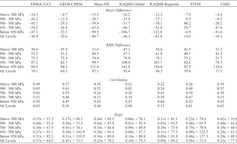
Table 5 shows statistics for these layers. The greatest mean differences (Table 5a) and RMS differences (Table 5b) occur in the lower levels. This is expected since many plumes are located relatively near the surface. It was shown earlier that the models have difficulties in these regions of enhanced CO. The correlations (Table 5c) show mixed results. Overall, the models tend to be less correlated with observations in the upper levels and moderately correlated with observations in the middle to lower levels. For example, the greatest correlations for the finer resolution models (RAQMS-Regional, STEM, UMD CTM), with the exception of Meso-NH, generally occur below 850 hPa. Each regional model, excluding Meso-NH, produces the worst correlations above 300 hPa. These small correlations could indicate that the regional models are unable to simulate the meteorological ascent that is needed to pump CO from its source regions at the surface to the upper levels. However, in general, statistics show that global CTMs present better correlations above 300 hPa than regional models. Therefore since CO at higher altitudes is more influenced by sources outside of the immediate TRACE-P region, this may cause difficulties for the regional CTMs. The unique behavior of Meso-NH is thought to result from its internal chemistry formulations, as discussed in section 2.1.

[40] We also examined very thin layers throughout the

atmosphere (978 – 976 hPa, 908 – 906 hPa, 728 – 726 hPa, 606 – 604 hPa, 428 – 426 hPa and 328 – 326 hPa) to determine if part of the models’ overall correlation (Table 3) was due to changes in altitude. These six layers were selected because they contained the greatest number of sampling points. The results (not shown) do not indicate large differences from the

correlations obtained over all levels (Table 3a). For example, correlations for GEOS-CHEM range from 0.40 to 0.83, versus a composite mean for all levels of 0.56. The best correlation (0.83) is at the 728 – 726 hPa level, and the worst (0.28) is for the 328 – 326 hPa level, similar to the findings for the deeper layers discussed above (Table 5). Similar results are observed for the other models.

4. Meteorological Processes

4.1. Composite Distributions

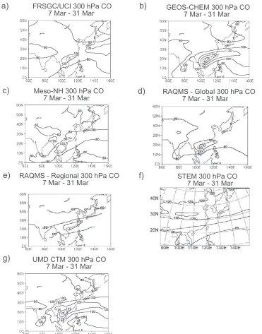
[41] Horizontal distributions of CO averaged over the

[image:10.592.52.540.91.388.2]

TRACE-P period provide a useful intercomparison of model results. The models best agree on the placement and inten-sity of CO at low levels, i.e., close to the surface-based emission sources. Figure 4 compares spatial fields of CO at 850 hPa for the period 7 – 31 March, the dates encompassing DC-8 flights 7 – 17. The greatest model-derived CO is over eastern India, in the same region as strong biomass burning and biofuel emissions (Figure 1). There is a second area of enhanced simulated CO over Southeast Asia where strong biomass burning emissions are located. This pattern is similar at 700 hPa (not shown), although Meso-NH no longer shows the maximum over Southeast Asia. In the upper levels, e.g., at 300 hPa (Figure 5), all models show similar distributions, reflecting convective pumping over Southeast Asia, followed by long-range eastward transport over the Pacific. However, the overall intensity of CO varies widely among the models. The two CTMs using closely related meteorological input data, GEOS-CHEM and UMD CTM, exhibit very similar results, and generally produce Table 5. Mean Difference of CO, RMS Difference, Correlation, and Slope for Five Atmospheric Layers and the Entire Vertical Column for the Combination of DC-8 Flights 7 – 17

FRSGC/UCI GEOS-CHEM Meso-NH RAQMS-Global RAQMS-Regional STEM UMD

Mean Difference

Above 300 hPa 14.7 0.7 13.5 26.2 12.5 7.5 6.4

500 – 300 hPa 26.2 12.9 20.7 35.8 37.1 0.3 6.3

700 – 500 hPa 43.1 20.3 39.9 51.7 58.1 40.2 20.2

850 – 700 hPa 54.2 36.8 65.4 80.7 81.8 29.7 47.6

Below 850 hPa 47.1 22.3 99.5 106.7 121.8 6.9 81.4

All Levels 36.9 20.6 49.7 56.3 61.8 14.6 34.3

RMS Difference

Above 300 hPa 38.6 45.5 31.6 47.1 38.8 41.5 31.2

500 – 300 hPa 53.2 52.5 49.5 67.1 61.9 48.1 41.3

700 – 500 hPa 75.5 75.4 74.4 78.0 78.1 75.1 51.7

850 – 700 hPa 87.2 82.7 99.7 108.0 101.7 82.6 78.3

Below 850 hPa 88.9 94.3 131.4 142.8 154.6 82.5 110.6

All Levels 70.1 69.5 87.1 91.4 96.3 70.8 71.1

Correlation

Above 300 hPa 0.49 0.37 0.58 0.21 0.22 0.26 0.55

500 – 300 hPa 0.65 0.61 0.52 0.02 0.24 0.48 0.57

700 – 500 hPa 0.65 0.53 0.24 0.20 0.61 0.59 0.58

850 – 700 hPa 0.51 0.46 0.32 0.18 0.59 0.47 0.53

Below 850 hPa 0.59 0.45 0.45 0.47 0.64 0.52 0.65

All Levels 0.65 0.56 0.44 0.48 0.51 0.61 0.62

Slope

(11)

greater CO values than the other models. These results suggest that model output, especially where removed from source regions, is highly dependent on the choice of mete-orological input data.

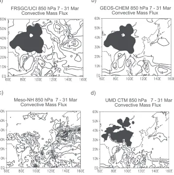
[42] Deep convection is the principal transporter of

emis-sions from the low levels into the upper troposphere. Therefore the placement and intensity of convective mass flux can greatly affect model results. Figure 6 compares distributions of convective mass flux at 850 hPa for 7 – 31 March. RAQMS and STEM did not report 3-D fields of convective mass flux; thus their data are missing from the figures. Each model shows relative maxima over eastern India, Southeast Asia, and the equatorial Pacific, agreeing with lightning data from the Lightning Imaging Sensor (LIS)

[image:11.592.115.483.63.530.2]

(available at http://thunder.msfc.nasa.gov) (Figure 7a) and precipitation patterns from Tropical Rainfall Measuring Mission (TRMM) (available at http://trmm.gsfc.nasa.gov) Merged Precipitation data (Figure 7b). On the other hand, Meso-NH shows comparatively weak cloud mass flux over Southeast Asia. Greatest differences among the models are found between 30 and 40N just east of Japan. Although each model shows enhanced cloud mass flux in this region, FRSGC/UCI and Meso-NH produce larger areas of enhance-ment and much stronger intensities. The TRMM rainfall totals appear to be greater in this region than over India and Southeast Asia, and there is lightning east of Japan. The results suggest that Meso-NH and FRSGC/UCI give the most realistic results between 30and 40N when compared

(12)

with TRMM rainfall and lightning data. The weak fluxes in the GEOS DAS are consistent with its tendency to underes-timate convection within midlatitude marine storm tracks [Allen et al., 1997].

[43] In the upper levels, e.g., at 500 hPa (Figure 8), the

models show similar patterns of convective mass flux over the equatorial Pacific, central Asia (30– 40N), and eastern India. However, compared with the other models, FRSGC/ UCI produces weaker mass flux over eastern India and much stronger values over Central Asia. It should be noted, however, that the FRSGC/UCI convective mass flux includes, in addition to convection, dry deposition and low-level turbulence. These near-surface effects, rather

than deep convection, seem to cause the much stronger values over Central Asia. In addition, GEOS-CHEM and UMD CTM continue to produce enhanced cloud mass flux over Southeast Asia, a feature not seen at these levels in the other models. We will examine these models’ convective mass flux in relation to CO error in section 4.4.

4.2. Pathways of Model CO Error

[44] One of our objectives is to investigate the

mecha-nisms by which the different CTMs, with their individual meteorological input data, simulate the outflow of CO from East Asia during TRACE-P. We specified thresholds to identify locations of significant differences between

[image:12.592.114.485.63.536.2]

(13)

eled and aircraft-derived CO and in a later section will investigate possible causes for these differences. Our thresh-olds were that modeled CO must be (1) 50 ppbv greater than or (2) 100 ppbv less than the measured values. The larger negative threshold is a result of the overall negative bias in model versus aircraft-derived CO.

[45] CO error varies somewhat among the models, but

trajectories based on FRSGC/UCI CO data are typical of the seven models. Composite 5-day backward trajectories for DC-8 flights 7 – 17, based on FRSGC/UCI CO error, are shown in Figure 9. Figure 9a shows trajectories from flight track arrival points where modeled CO exceeds the mea-sured value by 50 ppbv, whereas Figure 9b shows trajectories where modeled CO is less than the measured by at least 100 ppbv. Compared with measured CO, the FRSGC/UCI values are smaller by 100 ppbv (9.6% of total points) more often than they are larger by 50 ppbv (3.6% of total points). Nonetheless, these errors greater than +50 ppbv or smaller than 100 pbbv only represent a small fraction of all the points that were sampled (13.2%). The top panel shows a horizontal perspective, while the lower panel provides pressure altitude versus longitude. The color scheme indicates trajectory altitude, where warmer colors

denote trajectories at relatively high altitudes. Small arrows along the trajectory paths indicate locations at one-day intervals. An ‘‘x’’ at the end of a trajectory indicates that the parcel has exited the data domain before completing the 5-day period. Conversely an asterisk ‘‘*’’ indicates that the trajectory has completed the 5-day period inside the data domain.

[46] Trajectories of model CO errors greater than +50 ppbv

(Figure 9a) mostly show air that has traveled over Africa, India, and southern Asia before arriving at flight tracks south of 35N latitude in the mid levels (<700 hPa, >10,000 feet). A smaller number of trajectories originate over the South China Sea at lower levels, first traveling westerly before turning easterly where they reach the flight track. Deep convection is near both sets of trajectories over India and Southeast Asia. Section 4.4 examines how individual models handle this convection, to determine if this is a cause of discrepancy between models and aircraft-derived CO.

[47] For locations where the FRSGC/UCI model-derived

[image:13.592.121.474.70.426.2]

CO is at least 100 ppbv too small (Figure 9b), trajectories exhibit two major pathways: those arriving from the north-west and those arriving from the north-west. In addition, a relatively small number of trajectories arrive from the central

(14)

Pacific, and many also originate over the South China Sea, paths seen less often in the +50 ppbv CO error threshold. Parcels arriving from the west exhibit a similar pathway to the 100 ppbv threshold, traveling over Africa, India, and southern Asia; however, they arrive in the upper levels (300 hPa,30,000 feet). Significant convection is not seen near trajectories arriving from the northwest, but the air does travel over heavily industrialized regions (e.g., Shanghai).

4.3. Plume Displacement

[48] Discrepancies in location between simulated and

measured plumes are a limitation of current CTMs (Table 3b). Figure 10 shows horizontal distributions of CO at 250 hPa. At 0000 UTC on 27 March (Figure 10a), an area of enhanced CO is seen over eastern China; it moves over southern Japan by 0600 UTC (Figure 10b). The plume is relatively small in size and contains large horizontal gradients. Peak values of this feature are at 0400 UTC, just as DC-8 flight 15 passes through it, near 125E. Thus the model produces the plume of enhanced CO; however, there is a small shift in its simulated location compared with its observed location. Therefore the aircraft measures a

value of 229 ppbv whereas FRSGC/UCI provides 111 ppbv, even though the model’s nearby peak value is160 ppbv. These small shifts in plume location are observed in each of the CTMs throughout the TRACE-P simulations. A survey of other plume events (not shown) indicates that fine horizontal resolution models often simulate the plumes closer to their measured locations than models with coarser horizontal resolution.

4.4. Convective Outflow

[49] Insoluble gases such as CO are transported

[image:14.592.144.455.77.274.2]

verti-cally within convection with negligible loss [Allen et al., 1996b], and with a relatively long lifetime they can travel long distances from the convection. A major objective of DC-8 flight 15 (Figure 10) was to sample middle and high level outflow from intense distant convection over South-east Asia and China. The DC-8 took off from Yokota (36N, 139E), flew southwest to 23N, 133E, then headed west to 25N, 125E, and finally north over the Yellow Sea (37N, 125E). The Yellow Sea leg was designed to sample convective outflow at all levels south of 30N. The DC-8 then backtracked to 33N, 125E,

(15)

returning to Yokota around Korea and through the Sea of Japan. Figure 11 shows FSU 5-day backward trajectories for all points along the flight track.

[50] Figure 12 shows Geostationary Meteorological

Sat-ellite (GMS) 5 infrared imagery at the time of the flight (0631 UTC 27 March) (Figure 12a) and two days earlier (0631 UTC 25 March) when the trajectories (Figure 11) are near areas of deep convection over Southeast Asia. At flight time (Figure 12a), relatively weak convection is located south of Japan in the region of the flight path, while 2 days earli er (Figure 12b), strong storms are over Southeast Asia and along the east coast of China.

[51] Using the same technique as in the previous section,

i.e., trajectory thresholds based on model versus observed CO error, we next investigate the effects of these convective regions on model results. Figure 13 shows 5-day backward trajectories for DC-8 flight 15, based on CO errors from GEOS-CHEM. Trajectories arriving at points along the flight track where modeled CO exceeds the measured value by 50 ppbv (Figure 13a) originate from the west. Con-versely, trajectories arriving at points where modeled CO is less than the measured value by 100 ppbv (Figure 13b) originate from the northwest. These results are similar to those of the composite 5-day backward trajectories for Flights 7 – 17 combined, based on FRSGC/UCI CO error (Figure 9).

[52] GEOS-CHEM (Figure 13b) and the other six models

(not shown) produce CO errors of 100 ppbv in locations where trajectories arrive from the northwest. These trajectories do not encounter regions of significant convection along their paths (Figure 12), but the air does travel over highly industrialized regions (e.g., Shanghai). The similar CO errors among the models suggest that insufficient emissions may be a cause for the discrepancies between measured and modeled CO. In addition, the models’ difficulties in simulating the plumes that are often downwind of these industrialized areas, also may be a factor in causing the differences.

[53] Trajectories arriving from the west (Figure 13a) are

[image:15.592.115.481.60.414.2]

quite different. The simulated versus measured CO errors for GEOS-CHEM are larger than those of the other six models. To examine this difference, meteorological data from FRSGC/UCI and GEOS-CHEM are investigated in the convective regions. FRSGC/UCI was chosen because its simulated CO was within ±10 ppbv of measured values at all trajectory points, whereas GEOS-CHEM exceeded mea-sured values by 50 ppbv. Convective mass flux from FRSGC/UCI and GEOS-CHEM was interpolated to those trajectory paths where the GEOS-CHEM CO error exceeds measured CO by50 ppbv (Figure 13a). Convective mass flux at 6 hourly intervals for six representative trajectories is shown in Figure 14. The color of the lines indicates the

(16)

specific trajectory. Thus each color is used in two lines indicating the same starting point along the flight track (one line for GEOS-CHEM and the other for FRSGC/UCI). Dashed lines represent results from FRSGC/UCI, while solid lines show plots from GEOS-CHEM. The limitations of this methodology must be acknowledged. Convection reduces air mass integrity since updrafts and downdrafts within the convective column will mix air masses of different histories. Thus one can be confident in a trajectory reaching an initial convective area but less certain about

any prior paths or convective encounters. Nonetheless, we believe this approach provides informative results.

[54] Figure 14 reveals large differences in convective

[image:16.592.123.479.75.577.2]

mass flux between FRSGC/UCI and GEOS-CHEM. One should recall that the FRSGC/UCI (GEOS-CHEM) convec-tive mass fluxes are from the ECMWF (GEOS DAS). From flight time until 36 hours back, most trajectories travel over water (Figure 13a) where there are no emissions. However, the trajectories indicate air traveling near convec-tive regions of Southeast Asia at 42 hours back in time

(17)

and over eastern India at60 hours previous. Large differ-ences in convective mass flux are seen during both encoun-ters. These differences are important because there was significant biomass burning in these regions (Figure 1). The stronger convective mass flux of GEOS-CHEM (solid lines) provides more meteorological lift for these emissions to enter the free troposphere. This enhanced lift over Southeast Asia and eastern India may be the reason why the GEOS-CHEM-derived CO exceeds measured values by

50 ppbv at these points along flight 15. Conversely, FRSGC/UCI, with weaker convective mass flux, simulates CO within ±10 ppbv of aircraft-derived values.

[55] Distributions of convective mass flux at 850 and

500 hPa on 25 March at 0600 UTC for GEOS-CHEM and FRSGC/UCI (Figure 15) show that the results described in Figure 14 are representative for this particular flight. Con-vective mass flux from GEOS-CHEM is much stronger than from FRSGC/UCI at all levels over Southeast Asia and eastern India. However, GEOS-CHEM does not exhibit a systematic bias in overestimating convective mass flux for all DC-8 flights. Referring back to convective mass flux for the period 7 – 31 March (Figures 6 and 8), GEOS-CHEM’s results generally are similar to the other models. Therefore it is thought that DC-8 flight 8 is a particular case when GEOS-CHEM overestimates the convection, and is not a consistent problem with the model. This result is in contrast withAllen

et al.[1997], who showed that an earlier version of GEOS DAS (GEOS-1) overestimated the frequency and extent of convection in subtropical regions such as Southeast Asia. As stated previously, a major objective of this flight was to sample intense distant convection. The intensity of this convection is thought to be a cause of GEOS-CHEM’s overestimation. These results emphasize the importance of convective mass flux in chemical transport models.

4.5. Boundary Layer Depth

[56] Boundary layer depth plays an important role in

either capping or ventilating surface based pollutants. A major objective of DC-8 Flight 13 (Figure 16) was to sample dust and pollution outflow near the China coast. The DC-8 departed Yokota, Japan, flew southwest and crossed a weak front, then northwest recrossing the front, and finally north over the Yellow Sea before returning to Yokota. The leg over the Yellow Sea was within the boundary layer. Considerable Asian pollution was encoun-tered along this leg, including a well-defined crossing of the Shanghai plume near 29N where measured CO reached 1240 ppbv (Figure 3c).

[57] Figure 17 is a time series focusing on the Shanghai

[image:17.592.52.291.66.395.2]

plume, including aircraft altitude, measured CO, and the seven model-derived values. It is a close-up of a portion of Figure 3c. Although each model locates the intense Shang-hai plume within1latitude, they greatly underestimate its intensity. Vertical cross sections of CO along the northern leg of flight 13 are shown in Figure 18. Results from the STEM mesoscale CTM (Figure 9a) and the GEOS-CHEM global CTM (Figure 18b) illustrate these models’ simulation of this intense event. Both CTMs produce areas of enhanced CO near the surface from 25N to 34N. However, the intensity and exact placement of these areas vary. Horizon-tal distributions of CO at flight time, 0600 UTC 21 March (Figure 19), reveal that the enhanced region consists of two distinct plumes. The northern maximum (30N) represents the Shanghai plume, while the southern portion (26N) represents outflow from southern China. Although both plumes are located in eastern China, their vertical structures are quite different (Figures 18 – 19). The Shanghai plume is shallower (950 hPa versus 700 hPa) and has slightly greater CO than the southern plume.

[58] We investigated flow patterns and vertical thermal

stratification to determine possible causes for the plumes’ differing altitudes. The relatively weak front in Figure 16 is orientated northeast to southwest off the China coast. At the site of the Shanghai plume, there is a weak stable layer associated with the front at 850 hPa (not shown). This height corresponds closely to the top of the aircraft-docu-mented haze layer near the Shanghai plume (800 hPa,

7000 feet). A large anticyclone over Asia produces the offshore flow that dominates eastern China during most of the cold season [Fuelberg et al., 2003]. And, the postfrontal winds act to reinforce this eastward flow.

[59] The models’ boundary layer depth was examined

near the plumes, with PBL heights from GEOS-CHEM shown in Figure 20. The PBL height ranges from 950 to 925 hPa over eastern China and the Yellow Sea. Thus the PBL appears to cap the Shanghai plume. That is, surface emissions are prevented from being transported higher into the free troposphere. On the other hand, the southern plume,

(18)

extending to700 hPa (Figures 18 – 19), extends consider-ably higher than the shallow PBL.

[60] Horizontal distributions of CO two days prior to

flight time (0600 UTC 19 March, Figure 21) show origins of the two plumes. The Shanghai plume is a localized feature that originates near this coastal city. However, the southern plume does not appear to be localized. Instead, horizontal advection of CO occurs at all levels up to 700 hPa. Thus this area of enhanced CO seems to have been transported vertically near its source at some earlier time and therefore was not affected by the locally low PBL near the China coast. Conversely, PBL depth is very important to the Shanghai plume because it is produced by local emissions. The models do a good job of simulating the shallow PBL near Shanghai. Therefore the underesti-mation and spatial smoothing of local Shanghai emissions within the models appear to be the cause of the discrepancy between model-derived and simulated results.

5. Summary and Conclusions

[61] NASA’s Transport and Chemical Evolution over the

Pacific (TRACE-P) experiment, conducted between Febru-ary and April 2001, sought to characterize the chemical composition of Asian outflow and describe its evolution over the Pacific Basin. In addition to in situ chemical measurements by two NASA aircraft (a DC-8 and P-3B), TRACE-P included a major support activity from several

3-D chemical transport models (CTMs) that were used in real time to optimize flight strategies. This paper has described an intercomparison and evaluation of CO from seven 3-D CTMs that were run during TRACE-P. Each of the six modeling groups provided special post-mission simulations for the intercomparison, using the same com-mon set of emissions data.

[62] We first statistically analyzed the aircraft-derived and

seven numerically derived versions of CO. Values of model simulated CO were interpolated to the locations, altitudes, and times along each of the DC-8 flight tracks where measurements were made. The collocated measured and simulated values were used to calculate mean differences, RMS differences, correlations and slopes.

[63] The results for combined DC-8 flights 7 – 17

[image:18.592.115.478.78.395.2]

showed that values of model simulated CO generally were similar to measured values for the smaller values of CO, but they tended to diverge at greater values. The models showed an overall negative bias, with mean differences from measured values ranging from 67.3 to 14.6 ppbv. This negative bias may reflect an underestimate of the prescribed CO emissions sources. Correlations for the four global models ranged from 0.56 to 0.75, while correla-tions for the three regional models ranged from 0.44 to 0.61. Statistics from the global models did not differ greatly from those of the regional models, suggesting that increased model resolution does not necessarily produce better statistics with respect to measurements. However,

(19)

statistics for secondary plume pollutants such as photo-chemically produced ozone may show a different behav-ior with different model resolutions since averaging of fine-scale features in global models which are present in regional models, may lead to different net ozone produc-tion rates over a region.

[64] The statistical agreements varied greatly among the

individual flights. However, for each given flight, the models generally provided similar relative statistical results. Three flights were described in detail. DC-8 flight 8 was illustrated because its seven simulations were consistently among the best. Models produced RMS differences of

40 ppbv and correlations near 0.80. This flight exhibited

[image:19.592.132.475.87.293.2]

few spikes or plumes of CO. The models were most consistent in areas of relatively small CO. DC-8 flight 10 exhibited some of the greatest discrepancies among the models. Most models performed poorly, with correlations ranging from 0.13 to 0.71. Overestimating the amplitude of a midtropospheric CO peak, while greatly underestimating the amplitude of a boundary layer peak, was shown to be a limitation of some models. The model that produced the best correlation had fairly constant CO throughout the flight, which averaged out to the best result. The greatest measured CO occurred during flight 13 over the Yellow Sea. The various models generally did a good job of simulating CO for this flight. Each model correctly located

(20)

[image:20.592.117.473.115.667.2]

(21)

[image:21.592.115.479.242.487.2]

(22)

[image:22.592.118.477.64.418.2] [image:22.592.299.542.491.665.2]

Figure 15. Spatial fields of model-derived convective mass flux ( 10 3 kg/m2/s) for 0600 UTC 25 March; at 500 hPa (a) FRSGC/UCI, (b) CHEM and at 850 hPa (c) FRSGC/UCI, and (d) GEOS-CHEM. The dark areas denote regions where the surface pressure is below 850 hPa.

Figure 16. Flight track of DC-8 flight 13 (Yokota Local 1). The position of the cold front is shown by the long dashed lines.

[image:22.592.51.289.528.713.2]

(23)

[image:23.592.115.477.113.642.2]

(24)

[image:24.592.115.480.139.642.2]

(25)

the intense Shanghai plume that was sampled on two flight legs, but all models greatly underestimated its intensity.

[65] The models’ difficulties in simulating the intense

plumes during DC-8 flight 13 prompted further investiga-tion. We defined a plume using the criterion that the sampled air must exhibit CO values that were enhanced at least 20 ppbv above the local background. These results differed noticeably from those based on all measurements. For example, RMS differences generally were greater than 200 ppbv for plumes, versus a range from 41 to 128 ppbv for all segments. Discrepancies between simulated and measured plumes were due both to shifts in their physical placement and their magnitudes.

[66] We investigated whether there was a relationship

between CO error and altitude by dividing the atmosphere into five layers. Greatest mean differences and RMS differ-ences against measured values were found in the lower levels. This was expected since many plumes are located at these altitudes. Smaller correlations were found in the upper levels for most models. This indicates that the models may be unable to simulate the meteorological ascent that is needed to pump CO from its source region at the surface to the upper levels ate correct times and locations. Also, since CO at higher altitudes is more influenced by sources outside of the immediate TRACE-P region, this may have caused difficulties for the regional CTMs.

[67] We next investigated the mechanisms by which the

different CTMs, with their differing meteorological input data, simulated the outflow of CO from East Asia during TRACE-P. Three-dimensional model-derived CO data at 6 hourly intervals were provided for the entire TRACE-P period. Several modeling groups also provided parameters describing boundary layer processes and deep convection which could be compared with satellite imagery, rainfall totals, and lightning data.

[68] Horizontal distributions of CO averaged over the

TRACE-P period provided a useful intercomparison of model results. The models best agreed on the placement and intensity of CO at low levels, i.e., close to the surface-based emission sources. In the upper levels, e.g., 300 hPa, all models showed similar distributions; however, the over-all intensity of their CO varied widely. The two CTMs that used closely related meteorological input data exhibited very similar results. This finding suggests that model output, especially where removed from source regions, is highly dependant on the choice of initial meteorological input data.

[69] Thresholds were specified to identify locations of

significant differences between modeled and measured CO. Five-day backward trajectories based on model CO error were calculated for the combination of flights 7 – 17. Using results from FRSGC/UCI as a representative example, trajectories from those points along the flight tracks where model CO error exceeded the measured value by50 ppbv were found to arrive generally from the west. Conversely, trajectories of model CO errors 100 ppbv more often arrived from the northwest.

[70] DC-8 flight 15 was investigated to determine

possi-ble causes for differences between model and aircraft-derived CO. Using results from GEOS-CHEM as an example, trajectories from this flight showed similar paths as those for the combination of DC-8 flights 7 – 17. That is, trajectories arriving at points where GEOS-CHEM CO was less than the measured CO by 100 ppbv originated from the northwest. These parcels had traveled over heavily industrialized areas, including Shanghai. Since each of the seven models produced similar CO errors for these points, insufficient CO emissions may be a cause for the under-estimates. Trajectories arriving at points along the flight track where modeled CO exceeded measured CO by

50 ppbv originated from the west, having traveled over areas of deep convection in Southeast Asia and eastern India. Only one model produced CO exceeding the mea-sured value by 50 ppbv for these points along the flight track. This model was found to have much stronger con-vective mass flux than the other models near Southeast Asia and eastern India. Strong biomass burning was located in both areas at the time. Thus the strong convective mass flux in regions of strong emissions may have caused the model to produce CO that exceeded the measured values.

[71] DC-8 flight 13 was investigated to examine

meteo-rological processes affecting the models’ simulation of the intense Shanghai plume. The Shanghai plume was found to be a localized feature originating near that city. A large anticyclone over Asia was responsible for offshore flow that dominated the region. The models’ simulated PBL ranged from 950 to 925 hPa over eastern China and the Yellow Sea. The PBL was shown to cap the Shanghai plume, confining heavy pollution to the very lowest levels. A nearby second-ary area of enhanced CO, reaching 700 hPa, was not affected by the local PBL values. Unlike the Shanghai plume, this enhanced CO was transported aloft at some distant location and therefore was not influenced by the PBL in eastern China.

[72] Although this study did not consider the chemistry of

[image:25.592.51.285.67.318.2]

the seven CTMs, those aspects undoubtedly played a role in producing CO differences among the models and compared

(26)

[image:26.592.114.481.145.632.2]