Modeling Investment Cycles: A Theoretical Analysis

(1)

http://dx.doi.org/10.4236/me.2016.73037

How to cite this paper: Dalla, E., Karpetis, C. and Varelas, E. (2016) Modeling Investment Cycles: A Theoretical Analysis. Modern Economy, 7, 336-344. http://dx.doi.org/10.4236/me.2016.73037

Modeling Investment Cycles: A

Theoretical Analysis

Eleni Dalla1*, Christos Karpetis2, Erotokritos Varelas1# 1_{Department of Economics, University of Macedonia, Thessaloniki, Greece}

2_{Department of Balkan, Slavic & Oriental Studies, University of Macedonia, Thessaloniki, Greece}

Received 19 February 2016; accepted 22 March 2016; published 25 March 2016

This work is licensed under the Creative Commons Attribution International License (CC BY).

http://creativecommons.org/licenses/by/4.0/

Abstract

This paper establishes a second order accelerator model (Hillinger [1][2]) in discrete time. More specifically, we present a three-equation structural model in order to examine the behavior over time of capital. Our purpose is the analysis of investment cycles, defined as the quasi-periodic cyc-lical motion of capital. It is demonstrated that when the trigonometric oscillation is the case, the system is dynamically stable. In addition, we extend the analysis, introducing an exogenous credit term, the interest rate on loans, as an unknown function of time in the behavioral equation of in-vestors. We infer that the introduction of this credit term results in an alternative equilibrium level of capital.

Keywords

Investment Cycles, Second Order Accelerator, Capital, Exogenous Credit Term

1. Introduction

Business cycles are eminently dynamic phenomena to which many definitions have attributed. Generally, they are considered as periodic but irregular fluctuations in economic activity measured in terms of GDP or other macroeconomic variables. According to Zarnowitz [3], business cycles are characterized by persistence and pervasiveness. The former is related to the magnitude and the regularity of the economic disturbances while the latter refers to the existence of correlation among the macroeconomic variables.

Several classifications of business cycles theories can be found in the macroeconomic literature. For instance, Phelps [4] distinguishes seven schools while Arnold [5] divides them into five schools, namely Keynesian Eco-nomics, Monetarism, New Classical Economics, Real Business Cycles and NewKeynesian Economics. Our

(2)

terest is on the Keynesian Economics[6] according to which the determination of the investment cycle is based on the relation of the existing capital stock to the demand for output. In fact, this is the intuition behind the “ac-celerator principle”. The first multiplier-ac“ac-celerator model was established by Samuelson [7]. This analysis con-stituted a starting point for several recent researches. Westerhoff [8] extended the previous model, introducing a non-linear mix of extrapolative and regressive expectation formation mechanism. In this manner the model is useful for the implementation of economic policy as well. Karpetis and Varelas [9] introduced both the money market and the balanced government budget constraint in Samuelson’s model. An extension of the Samuelson multiplier-accelerator model was also proposed by Dassios, Zimbidis and Kontzalis [10] who incorporated de-layed variables in the initial model. Their analysis achieves to interpret the origination of stable business cycles if realistic and stochastic values of both the multiplier and the accelerator are concerned. Following a similar approach, Dassios and Zimbidis [11] studied the stability of the national economy in the case of an interaction among different countries. Moreover, Puu, Gardini and Sushko [12] presented a Hickian type [13] model that concentrates on the “floor” of income and omits the “ceiling”. This model interprets the existence of business cycles with increasing amplitude. Puu [14] extended the previous model, introducing the “ceiling” of income as well.

Although the theoretical models in this field generate investment cycles and suggest that the roles of con-sumption and investment are of the same importance, this suggestion is not confirmed by the empirical observa-tions. In fact, the latter imply that investment is more sensitive to the business cycle than the consumption. Hil-linger [1] developed a model in continuous time, explaining the central role of investment and inventory deci-sion. Indeed, the fact that short run adjustments occur in quantities, not in prices, is a basic assumption of the theory of investment cycles and marks a great divide to the neoclassical paradigm. Hillinger, Reiter and Weser [15] derived the second order accelerator for both fixed investments and inventories, regarding the microeco-nomic firm behavior. Hillinger and Weser [16] and Weser [17] used the second order accelerator model to dis-cuss the aggregation problem that arises in business cycles theory. In the same manner, Woitek [18] and Barnett, Gandolfo and Hillinger [19] examined the business cycle stylized facts following an empirical approach. This ability of the second order accelerator models to comply with the stylized facts, which imply a major role for investment in the fluctuations of economic activity, makes them a very important mechanism of interpreting in-vestment cycles.

In this paper, we propose a second order accelerator model in discrete time as a mechanism to provide an ex-planation of the endogenous origination of investment cycles. The significance of the research lies in the intro-duction of the monetary term, which allows the investigation of the effect of the structure of the banking sector on the investment cycle in the long run. Therefore, following Hillinger [1] [2], we present a three-equation second order accelerator model in discrete time. In addition, we incorporate an exogenous credit term, the inter-est rate on loans, which is an unknown function of time. Our purpose is dual. On one hand, we attempt to in-terpret the existence of investment cycles. On the other hand, we are interested in the implications of the intro-duction of the interest rate on loans on the time path of capital.

The paper is structured as follows. Firstly, we discuss the theoretical model. Then, the solution of the model and the stability conditions of the system are presented. The next section shows a graphical location of the roots. Section 5 introduces the exogenous interest rate on loans into the fundamental behavioral equation of invest-ment. Section 6 concludes.

2. The Three-Equation SOA Model in Discrete Time

We derive the Second Order Accelerator (SOA) of net investment in discrete time, using the standard flexible accelerator [1]. This model provides a behavioral explanation of the investment cycle. In addition, it takes into consideration the time interval between the investment decision and its transformation into capital. Our structur-al model is described by the following set of difference equations:

(

*

)

1 1 , 0 1

t t t t

I I− − =c I −I− < <c (1)

(

)

* *

1 , 0

t t t

I =b K −K− b> (2)

1

t t t

(3)

338

Equation (1) constitutes the partial adjustment mechanism for net investments. It shows that the net invest-ment is adjusted towards the desired level of investinvest-ment ( *

t

I ) gradually. The coefficient c ∈ (0, 1) is the speed of adjustment. The closer to the unity is the value of c; the faster is the adjustment of net investment in the present period. On the contrary, as the value of c approaches zero, the adjustment becomes slower. The partial adjustment mechanism is based on the assumption of the existence of adjustment costs which are related to changes in the level of investment. Thus, if the adjustment costs are omitted from the model, the net investment is adjusted towards its desired level ( *

t

I ) perfectly, that is *_& ₁

t t

I =I c= .

Equation (2) is a behavioral equation. It expresses the desired level of net investment ( * t

I ) as a fraction of the difference between the desired level of capital ( *

t

K ) and the actual level of capital with a one-period lag (Kt−1). The constant b is positive, reflecting the positive relation between the desired level of net investment ( *

t I ) and the aforementioned difference. It should be noted that the introduction of the time pattern of the investment ex-penditure leads to a time lag in the transformation of this exex-penditure into capital. In particular, we follow the time-to-build and time-to-plan approaches according to which the costs of investment projects are incurred with time lags and become productive only when the project is complete. Undoubtedly the existence of adjustment lags is in no sense an indication of irrational behavior. There are costs incurred if the various lags are shortened and other costs if they are lengthened. Under the assumption of a finite time path, we presume that the desired level of capital is stable over time. This allows the notation of the desired level of capital with K*_{for the rest of} our analysis. Finally, Equation (3) is the definition of net investment. Net investment (It) is defined as the change in the stock of capital (K Kt− t−1).

3. Solution of the Model

Equations (1)-(3) constitute the structural form of our model. From their combination, we deduce the reduced form which is given by the following equation:

(

)

(

)

*

1 2

1 2 1

t t t

K +c b+ − K− + −c K− =cbK . (4)

Equation (4) presents the second order accelerator for net investment. Mathematically, it is a second-order difference equation with constant coefficients. The general solution of this non-homogeneous equation is de-rived adding the general solution of the corresponding homogeneous equation and any particular solution of the non-homogeneous Equation (4). To begin with the general solution of the homogeneous equation, it shows the deviation of capital from the equilibrium. The functional form of this general solution depends on the sign of the discriminant of the corresponding characteristic equation.

Taking into consideration that, the homogeneous equation, as this is obtained by (4), has the following ma-thematical form:

(

1 2

)

1

(

1

)

2 0

t t t

K +c b+ − K− + −c K− = , (5)

the corresponding characteristic equation is:

(

)

(

)

2 _{c b} _{1 2} ₁ _c ₀

λ +_ + − _λ+ − = , (6)

and the crucial for our analysis value of the discriminant of the characteristic equation is:

(

)

2

2 ₁ ₄

c b cb

∆ = + − . (7)

Therefore, three cases are possible.

Firstly, in the case of a positive discriminant, the characteristic equation possesses two real and linearly inde-pendent roots. Applying the Vieta’s formulas, it is inferred that these roots are of the same sign. Particularly, when these roots are positive, the time path of capital is monotonic. On the contrary, the negative sign of both roots implies improper oscillatory movement of capital. In any case, capital converges towards its long-run equilibrium if, and only if, both roots are less than unity in absolute values. Otherwise, capital diverges from its equilibrium.

(4)

339

value of the characteristic root is less than unity. On the contrary, if the characteristic root is greater than unity in absolute values, capital diverges from the long-run equilibrium. Regarding the kind of this movement, the con-vergence will be monotonic if the value interval of the characteristic root is the (0, 1), while it will be improper oscillatory if the value interval is the (−1, 0). Similarly, the divergence will be monotonic if the value of the characteristic root belongs to the interval (1, +∞), while it will be oscillatory if the value interval is (−∞,−1).

Finally, a negative discriminant implies two complex conjugate characteristic roots. In this case, capital shows trigonometric oscillations with period equal to 2π/ω and amplitude dependent on the modulus or absolute value (R) of the complex conjugate roots. After proper calculations, this modulus (R) is derived equal to R= 1−c. From the assumptions of our structural model concerning the value intervals of the parameters, it is deduced that the absolute value of the complex conjugate roots is less than unity. Consequently, capital converges towards its equilibrium, following a trigonometric oscillatory path with decreasing amplitude.

In any case, the stability of our system can also be ensured by the satisfaction of a set of necessary and suffi-cient conditions [20]. These conditions have as follows:

0

cb> (8)

0

c> (9)

(

2

)

4

c b+ < . (10) Therefore, it is inferred that the critical condition for the existence of dynamic stability is inequality (10). Moving now into the particular solution of the non-homogeneous Equation (4), this can be interpreted as the equilibrium level of capital. Applying the method of undetermined coefficients, we get:

* t

K =K (11)

Thus, the equilibrium level of capital is equal to capital’s desired level.

In conclusion, it has to be mentioned that our interest lies in the case of the trigonometric oscillatory move-ment of capital. For this reason we concentrate on the possibility of negative discriminant(Δ < 0). Hence, the general solution of the non-homogeneous difference equation (4) is given by the sum:

[

]

*

1cos 2sin t

t

K =R A ωt A+ ωt +K , (12) where Α1, Α2∈ℜ are arbitrary constants which can be derived using two initial conditions.

4. Graphical Positioning of the Characteristic Roots

In this section, we investigate the nature of the characteristic roots and the dynamic properties of our model for different values of the speed of adjustment parameter (c) and the behavioral parameter b. Thus, after making use of the discriminant (Equation 7) and the critical stability condition (Equation 10), we depict the following func-tions:

(

)

2

4 1 , 1

c= b b+ b≠ − (13) &

(

)

4 2 , 2

c= b+ b≠ − (14)

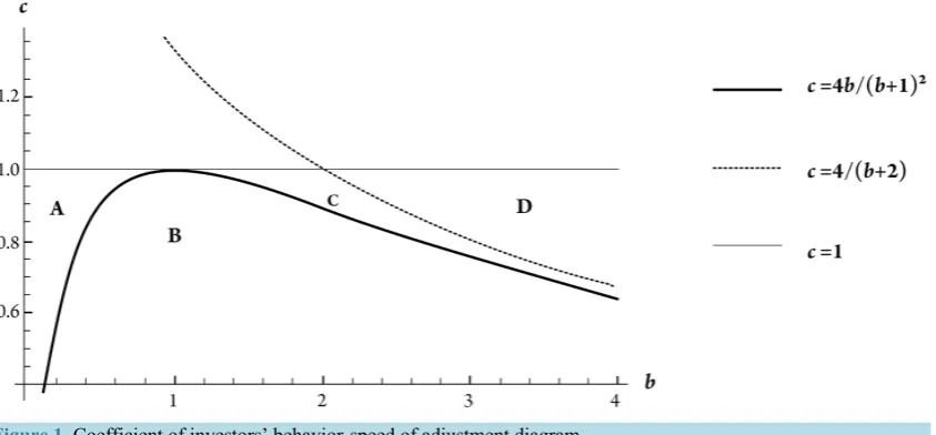
Figure 1 illustrates all the possible cases that were discussed in Section 3. The values of the parameter b and the values of the speed of adjustment c are shown on the horizontal and vertical axes respectively. The graphical representations of Equations (13) & (14) divide the two dimensional space into four distinct regions1_{, that is A,} B, C & D. Taking into consideration that c ∈ (0, 1) & b > 0, these regions include only the points of the first quadrant that lie below the line c = 1.

4

c b+ < . The former implies that the characteristic roots are real while the latter demonstrates the dynamic

1_{Given that} ₍ ₎2 ₍ ₎ ₍ _{) (}2 ₎

(5)

[image:5.595.106.528.86.282.2]

340

Figure 1. Coefficient of investors’ behavior-speed of adjustment diagram.

stability of the system. Therefore, capital converges towards its steady-state. In addition, the points of section B are allocated below both the functions (13) & (14). That is Δ < 0 and c b

(

+2

)

<4. The characteristic roots are complex and the crucial stability condition is satisfied. The result is a trigonometric oscillatory movement that converges towards the steady-state. Moving now to section C, the corresponding points lie above the function

(

* *

1 , 0, 0

t t t Lt

I =b K −K− +dr b> d< (16)

1

t t t

I =K K− − , (17) where c: the speed of adjustment; b: a parameter of investors’ behavior; d: a parameter that shows the negative relation between the interest rate on loans and the desired level of net investments; rLt: the exogenous interest rate on loans, the functional form of which is unknown.

(6)

stable over time as before. Consequently, it is denoted with K*_{for the rest of this section.}

After the combination of Equations (15)-(17), we obtain the second order accelerator for fixed investment:

(

)

(

)

*

1 2

1 2 1

t t t Lt

K +c b+ − K− + −c K− =cbK +cdr . (18)

Equation (18) is a second-order difference equation with constant coefficients. The solution of this equation requires the determination of the general solution of the corresponding homogeneous difference equation and the derivation of a particular solution of the non-homogeneous Equation (18). The homogeneous equation that is implied by (18) is:

(

1 2

)

1

(

1

)

2 0

t t t

K +c b+ − K− + −c K− = . (19)

Comparing Equations (5) and (19), we infer that the introduction of the exogenous interest rate on loans in-fluences neither the homogeneous equation nor the stability conditions. Thus, the deviation of the system from its equilibrium remains unaffected. What is influenced by the interest rate on loans is the particular solution of Equation (4), i.e. the equilibrium level of capital (dynamic equilibrium in this case).

Taking into consideration that the functional form of rLt is unknown; we apply the operational method to de-duce the particular solution of (18). The final outcome depends on the absolute value of the characteristic roots. More specifically, let λ1, λ2 denote the characteristic roots. To begin with the case of two real linearly indepen-dent roots, we have to distinguish between three subcases. Firstly, if λ λ₁, ₂ <1, the particular solution of (18) is:

( )

2

*

1 0

i

t n n Lt i

n i

K K cd θ ∞ λ r ₋

= =

= +

∑ ∑

, (20)

where

(

)

(

)

1 1 1 2 & 2 2 1 2

θ =λ λ λ− θ = −λ λ λ− .

This solution refers to the points that lie on the regions A and C of Figure 1. Indeed, the fact that λ λ1, 2 <1 implies that capital converges towards its equilibrium. Secondly, when λ λ1, 2 >1 the particular solution of (18) has as follows:

2 *

1 1

1 i

t n Lt i

n i n

K K cd θ r

λ

∞

+

= =

 

= − _ _

 

∑ ∑

, (21)

where

(

)

(

)

1 1 1 2 & 2 2 1 2

θ =λ λ λ− θ = −λ λ λ− .

Finally, if λ <j 1 & λk >1, with j, k = 1, 2 & j ≠k, then the particular solution becomes:

( )

*

0 1

1 i

i

t j j Lt i k Lt i

i i k

K K cd θ λ r θ r

λ

∞ ∞

− +

= =

 _ _ 

 

= + − _ _

   



∑

, (22)

where

(

)

&

(

)

j j j k k k j k

θ =λ λ −λ θ = −λ λ −λ .

0 1 0 1

i i

t Lt i

i i

K cb ∞ i λ K cd ∞ i λr ₋

= =

 

= _ + _ + +

(7)

342

Finally, under the existence of negative discriminant, the characteristic equation has two complex conjugate roots with absolute value less than unity. In fact, this corresponds to the points in the region B in Figure 1. Thus, the particular solution that is obtained is the following one:

( )

2

*

1 0

i

t n n Lt i

n i

K K cd θ ∞ λ r ₋

= =

= +

∑ ∑

, (24)

where

(

)

(

)

1 1 1 2 & 2 2 1 2

θ =λ λ λ− θ = −λ λ λ− .

Since the particular solutions (20)-(24) represent the equilibrium value of capital in each case, they should be positive. Specifically, in terms of relation (24), it should be hold:

( )

2

*

1 0

i

n n Lt i

n i

K cd θ ∞ λ r ₋

= =

> −

∑ ∑

. (25)

On the whole, the time path of capital for the case of trigonometric oscillatory movement is described by the following aggregate:

[

]

* 2

( )

1 2

1 0

cos sin i

t

t n n Lt i

n i

K R A ωt A ωt K cd θ ∞ λ r ₋

= =

= + + +

∑ ∑

, (26)

where Α1, Α2∈ℜ are arbitrary constants which can be derived using two initial conditions.

In the long-run the magnitude of economy’s physical capital is expected to converge to a diachronically con-stant equilibrium value, which cannot be different from the desired level of capital:

*

lim t t 0

t→+∞K =K =K > (27)

Taking the limit of relation (26) with t →∞ we have that:

( )

[

]

( )

[

]

* 2 * 1 2 1 0 2 * 1 2 1 0 0

lim lim cos sin

lim lim lim lim cos sin

i _t

t _t t _t n n Lt i

n i

i t

n n Lt i

t t _n _i t t

K

K K K cd r R A t A t

K cd r R A t A t

θ λ ω ω

+∞ − →+∞ →+∞ ₌ ₌ +∞ − →+∞ →+∞ ₌ ₌ →+∞ →+∞   = = _ + + + _     = + _ _+ × +  

∑ ∑

(

)

( )

2 * 1 0 i lim

t n n _t Lt

n i

K K cd θ +∞ λ L r

→+∞

= =

 

⇒ = +

∑ ∑

_ _ (28)

In the frame of relation (28), the physical capital will converge to a steady-state equilibrium value only when

{ }

r_{Lt t}+∞₌₀ is a bounded sequence, that is when _lim

( )

*

( )

_0,1

Lt L

t→+∞ r = ∈r , where

* L

r the constant equilibrium value of the exogenous interest rate on loans. In this case the aforementioned relation is transformed as follows:

(

)

2

)

2 2

1 2

0,1 , 0 & 1 1 1 0

c∈ d< −λ −λ = −m +n > , with m (n): the real (imaginary) part of the conjugate complex characteristic roots λ = ±_j m n i j, , =1, 2.

In the case of a perfectly competitive banking sector, the steady-state equilibrium value of the lending rate is expected to be non-negative, that is * ₀

L

r ≥ . In the special case where * ₀ L

r = , relation (30) is altered taking the following form:

* ₀

− =

t

K K or equivalently *

t

K =K (31) On the basis of relation (31), the necessary condition for the production of full employment income is the perfectly competitive structure of the economy’s banking sector.

The zero equilibrium value of the lending rate could be justified in the cases where, firstly, the competitive banking sector reaches a steady-state equilibrium with a long run average cost equal to zero at the optimum point (rL*= LAC = 0) and, secondly, the cash reserve ratio is set equal to zero by the monetary authorities.

6. Conclusions

In this paper, we attempted to interpret the existence of investment cycles, following the standard flexible acce-lerator. Our model extended the existing literature in the field of investment cycles, establishing a second order accelerator model in discrete time and introducing an exogenous monetary term. This extension allowed the in-vestigation of the implications of the structure of the banking sector on the long-run equilibrium of capital. In particular, we established a three-equation structural model, the reduced form of which presented the second or-der accelerator of net investment in discrete time. The latter was described by a second oror-der difference equation with constant coefficients. The solution of this equation yielded the behavior over time of capital. We concen-trated on the case of cyclical behavior of capital. Moreover, it was demonsconcen-trated that the equilibrium level of capital is equal to its desired level. The graphical representation of all the possible cases occurred showed that when the trigonometric oscillation is the case, capital converges towards its steady-state.

Finally, we proved that the introduction of the exogenous interest rate on loans in the behavioral equation of our structural model affects neither the deviation of capital from equilibrium nor the period of the oscillation in the case of trigonometric oscillatory movement. Additionally, the possibilities of convergence towards the long-run equilibrium are not influenced too. We concluded that when the equilibrium value of the lending rate is positive, the influence of the exogenous credit term lies in an alternative equilibrium level of capital.

This analysis raises three issues as subjects of future research. The first one is the investigation of the effects of the introduction of an endogenous monetary term in the three-equation second order accelerator model on the time path of capital. The second one concerns the implications of monetary policy in this context. The last one is related to the implementation of an empirical approach to examine the system’s ability to interpret the stylized facts in different countries.

References

[1] Hillinger, C. (1992) Cyclical Growth in Market and Planned Economies. Clarendon Press, Oxford.

[2] Hillinger, C. (2005) Evidence and Ideology in Macroeconomics: The Case of Investment Cycles. Munich Discussion Paper No. 2005-16. https://epub.ub.uni-muenchen.de/694/1/EANDIMUNICH.pdf

[3] Zarnowitz, V. (1992) What Is a Business Cycle? In: Belongia, M.T. and Garfinkel, M.R., Eds., The Business Cycle: Theories and Evidence, Proceedings of the 17th Annual Economic Policy Conference of the Federal Reserve Bank of St. Louis, Kluwer Academic Publishers, Boston, 4-72. http://dx.doi.org/10.1007/978-94-011-2956-5_1

[4] Phelps, E. (1990) Seven Schools of Macroeconomic Thought. Clarendon Press, Oxford.

http://dx.doi.org/10.1093/0198283334.001.0001

[5] Arnold, L. (2002) Business Cycle Theory. Oxford University Press, Oxford.

http://dx.doi.org/10.1093/acprof:oso/9780199256815.001.0001

[6] Keynes, J. (1936) The General Theory of Employment, Interest and Money. Macmillan, London.

[7] Samuelson, P. (1939) Interaction between the Multiplier Analysis and the Principle of Acceleration. Review of Eco-nomic Statistics, 4, 75-78. http://dx.doi.org/10.2307/1927758

(9)

344

http://dx.doi.org/10.1080/13504850500390663

[9] Karpetis, C. and Varelas, E. (2012) Fiscal and Monetary Interaction in a Simple Accelerator Model. International Ad-vances in Economic Research, 18, 199-214. http://dx.doi.org/10.1007/s11294-012-9345-4

[10] Dassios, I., Zimbidis, A. and Kontzalis, C. (2014) The Delay Effect in a Stochastic Multiplier-Accelerator Model. Journal of Economic Structures, 3, 7.

[11] Dassios, I. and Zimbidis, A. (2014) The Classical Samuelson’s Model in a Multi-Country Context under a Delayed Framework with Interaction. DiscreteandContinuous Dynamical System, Series B, Applied Algorithms, 21, 261-274. [12] Puu, T., Gardini, L. and Sushko, I. (2005) A Hicksian Multiplier-Accelerator Model with Floor Determined by Capital

Stock. Journal of Economic Behavior & Organization, 56, 331-348. http://dx.doi.org/10.1016/j.jebo.2003.10.008 [13] Hicks, J. (1950) A Contribution to the Theory of the Trade Cycle. Clarendon Press, Oxford.

[14] Puu, T. (2007) The Hicksian Trade Cycle with Floor and Ceiling Dependent on Capital Stock. Journal of Economic Dynamics and Control, 31, 575-592. http://dx.doi.org/10.1016/j.jedc.2005.12.004

[15] Hillinger, C., Reiter, M. and Weser, T. (1992) Micro Foundations of the Second-Order Accelerator and of Cyclical Behavior. In: Hillinger, C., Ed., Cyclical Growth in Market and Planned Economies, Clarendon Press, Oxford, 167- 180.

[16] Hillinger,C. andWeser,T. (1988) The Aggregation Problem in Business Cycle Theory. Journal of Economic Dynam-ics and Control,12, 37-40.

[17] Weser, T. (1992) The Aggregation Problem for Economic Cycles. In: Hillinger, C., Ed., Cyclical Growth in Market and Planned Economies. Clarendon Press, Oxford, 181-200.

[18] Woitek, U. (1995) Business Cycles: An International Comparison of Stylized Facts in a Historical Perspective. Physi-ca-Verlag, Heidelberg.

[19] Barnett, W., Gandolfo, G. and Hillinger, C. (1996) Dynamic Disequilibrium Modeling. Cambridge University Press, New York.