Efficient Numerical Methods for Solving Differential Algebraic Equations

http://dx.doi.org/10.4236/jamp.2016.41007

Efficient Numerical Methods for Solving

Differential Algebraic Equations

Ampon Dhamacharoen

Department of Mathematics, Burapha University, Chonburi, Thailand

Received 19 November 2015; accepted 8 January 2016; published 11 January 2016

Copyright © 2016 by author and Scientific Research Publishing Inc.

This work is licensed under the Creative Commons Attribution International License (CC BY).

http://creativecommons.org/licenses/by/4.0/

Abstract

This research aims to solve Differential Algebraic Equation (DAE) problems in their original form, wherein both the differential and algebraic equations remain. The Newton or Newton-Broyden technique along with some integrators such as the Runge-Kutta method is coupled together to solve the problems. Experiments show that the method developed in this paper is efficient, as it demonstrates that implementation of the method is not difficult, and such method is able to pro-vide approximate solutions with ease within some desired accuracy standards.

Keywords

Differential-Algebraic Equations, Newton-Broyden Method, Index-2 Hessenberg DAE

1. Introduction

A differential algebraic Equation (DAE) is an equation involving an unknown function and its derivatives. A DAE in its most general form is given by the following:

( ) ( ) ( )

(

t, t , t , ′ t

)

= , t∈

[ ]

a b,

F x y y 0 (1)

where R is the set of real number, F: R×Rm×Rn×Rn →Rm n+ , _x

( )

_t ∈Rm

, _y

( )

_t ∈Rn

and y′

( )

t ∈Rn. In this form, the relationship between the variables and derivatives may be implicit. In some systems, the equations may be written in the explicit form of derivatives, as follows:

( )

t

(

t,

( ) ( )

t , t

)

′ =

y f x y (2a)

( ) ( )

(

t, t , t

)

=

where : R_×Rm_×Rn_→Rn

f , This set of equations is called a semi-explicit DAE system.

Differential algebraic equations arise in the mathematical modeling of a wide variety of problems found in engineering and science, such as multi-body and flexible body mechanics, electrical circuit design, optimal con-trol, incompressible fluids, molecular dynamics, chemical kinetics and chemical process control [1]-[5].

DAEs can be transformed into ODE problems via differentiation. The number of differentiations needed in the transforming process is called the differentiation index. This number can describe some characteristics of the problem. In general, the higher the index of a DAE, the more difficulties one can expect in its numerical solution

[1]-[3] [6].

Although DAEs can be transformed into an explicit ODE so that it can be solved using the methods of ODE, there are still many numerical methods that can solve DAE directly. In the DAE solvers software, the numerical approaches for the solution of DAEs can be divided roughly into two classes: a) direct discretizations of the given system; and b) methods which involve a reformulation (e.g. index reduction), combined with a discretiza-tion. Direct discretizations are easier to use, but are limited in their utilitisation to essentially index-1, index-2 Hessenberg, and index -3 Hessenberg DAE systems, while a reformulation may be costly, and it may also re-quire more input from the user and involve more user intervention [3] [6].

In this research, we will place emphasis on constructing an algorithm for solving a semi-explicit DAE. The approach employed is to firstly solve the system of algebraic equations, and subsequently solve the differential equations using the derived information. The Newton-Broyden method plays a key role in solving algebraic eq-uations, since it performs almost as well as the Newton method, but requires less energy, and in addition, it also outperforms other methods of the same order of convergence [7]-[9].

2. The Newton-Broyden Method

The method, which was first proposed by Dhamacharoen in 2011 [7], [8], aims to solve the equation of the form:

( )

(

,

)

=

F u x x 0 (3)

The Newton scheme of this problem is:

( )

(

)

( )

(

( )

)

1

(

( )

)

1 , , , , 0,1, 2, .

i i i i i i i i i i

−

+ = − u ′ + x  =

x x F u x x u x F u x x F u x x  (4)

Replacing u x′

( )

i by Di, gives

( )

(

)

(

( )

)

1

(

( )

)

1 , , , , 0,1, 2, .

i i i i i i i i i i

−

+ = − u + x  =

x x F u x x D F u x x F u x x  (5)

with updating:

( ) ( )

(

)

T

1 T 1

1

i i i i i i i

i i

+ = − + − −

D D u x u x D b b

b b (6)

where bi = xi+1−xi. Equation (6) is called the Broyden rank-1 update, and (5) with the update (6) is called the

Newton-Broyden method. This method retains the good part of the Newton method, and replaces the difficult part of Newton’s with Broyden’s. With good initial guesses for z0 and D0, the Newton-Broyden Scheme (5) will

produce a sequence that converges to a solution of (3), with q-super linear order of convergence.

Although the order of convergence of the Newton-Broyden method is equal to that of the Broyden method, and less than that of the Newton method, in practice, the Newton-Broyden performs well in the sense that a good initial guess is easily found, and it reaches the solution in a reasonable number of ierations. As shown in [7] and

[8], for the same problem and using the same initial guess, the sequences from the Newton method and from the Newton-Broyden method reach the solution, while that from the Broyden does not. In addition, the New-ton-Broyden method requires less amount of work in comparison with the Newton method.

Note that if function F is linear, then Broyden’s update and Newton-Broyden’s update coincide.

3. Constructing the Method

Assume that the DAE is expressed in the form (2a), (2b) (renumbering)

( )

t

(

t,

( ) ( )

t , t

)

′ =

y f x y (7a)

( ) ( )

(

t, t , t

)

=

g x y 0 (7b)

( )

t0 = 0

y y (7c) in which the system of equations is to be solved for x(t) and y(t), where t∈ [a, b]. In solving the system numer-ically, the conditions on the initial values of y must be imposed sufficiently for the system to have a unique solu-tion. If (7b) can express x(t) in terms of t and y(t) explicitly, then the system becomes a pure ODE. Therefore, we consider the case when (7b) expresses x(t) implicitly.

Let the interval [a, b] be divided into n subintervals

{

a=t t0, ,1,t n= b

}

. In each interval

[

ti−1,ti

]

, we will

solve (7a) numerically for y

( )

ti . In an initial value problem, the value y

( )

t0 is specified, and the value

( )

t0

x can subsequently be solved from (7b). In order to use the Runge-Kutta method, in each interval

[

ti−1,ti

]

the value x1, x2 and x3, which are needed for computing F2, F 3 and F4 respectively, can each be solved

from (7b) using the values of y

( )

ti−1 +F1 2 in F2, y

( )

ti−1 +F2 2 in F3 and y

( )

ti−1 +F3 2 in F4. Once the

value y

( )

ti is computed, x

( )

ti can then be solved from (7b). Advance to the next interval, and repeat this

procedure until we reach the last subinterval.

Suppose the term x(t) is missing from the Equation (7b). Therefore, the system becomes:

( )

t

(

t,

( ) ( )

t , t

)

′ =

y f x y (8a)

( )

(

t, t

)

=

g y 0 (8b)

( )

t0 = 0

y y (8c)

in which the system is called index-2 Hessenberg. In solving the differential Equation (8a), the variable x(t) are treated as unknowns. In each interval

[

ti−1,ti

]

, the value of x

( )

ti−1 is given as a guess, and (8a) is then solved

numerically for y

( )

ti . Check the condition (8b) g

(

ti,y

( )

ti

)

=0. Update the value of x

( )

t0 and iterate the

process until the condition (8b) is met. Subsequently, advance to the next interval using the last value of x

( )

ti−1

as the guessing value for x

( )

ti . Repeat this procedure until we complete the last subinterval.

In solving the differential equations, we may use the 4th order Runge-Kutta method, or the 4th order Taylor method, since their local error is O

( )

h5 and the total error is O

( )

h4 , which is acceptable and also easy to im- plement. In solving the algebraic equations associated in the problem, the Newton method is used in (7b), and the Newton-Broyden method is used in (8b).

As per the procedure described above, the formulation will be as follows:

Partition the interval [a, b] into n subintervals. h b a n

−

= , and t0=a t, i=ti−1+h i, 1, 2,= , .n

Problem (7a), (7b):

Define the function F: F x

(

( )

ti−1

)

=g

(

ti,x

( ) ( )

ti ,y ti

)

, i=1, 2,,n.

The problem become (3)

( )

(

ti−1

)

=

F x 0

which can be solved using the Newton method. P1: Newton Method.

Prescribe a small positive real number ε. Guess the value z.

A: Compute F(z). Check if ||F(z)|| < ε

Solve the system F'(z)b = −F(z), for b. Set z = z + b.

Go to A. B: End.

The process for solving the DAE will be as follows: Algorithm A:

Initial step:

1) Set the given initial condition y

( )

t0 = y0.

2) Solve for x

( )

t0 , using P1: Set x

( )

t0 =z.

Main step:

For i=1, 2,,n; process the following steps:

Step 1. Solve the initial value problem (7a) 1 step to obtain y

( )

ti , by proceeding using the following steps:

1) Compute: F1=hf

(

ti−1,x

( ) ( )

ti−1 ,y ti−1

)

, y1= y

( )

ti−1 +F1 2, Solve g

(

ti−1+h 2 ,x y1, 1

)

=0 for x1.

(Using P1).

2) Compute: F2=hf

(

ti−1+h2 ,x y1, 1

)

( )

2= ti−1 + 2 2

y y F , Solve g

(

ti−1+h2 ,x2,y2

)

=0 for x2. (Using P1).

3) Compute: F3=hf

(

ti−1+h 2 ,x2,y2

)

( )

3 = ti−1 + 3 2

y y F , Solve g

(

ti−1+h,x y3, 3

)

=0 for x3. (Using P1).

4) Compute: F4 =hf

(

ti−1+h,x y3, 3

)

5) y

( )

ti = y

( )

ti−1 +

(

F1+2

(

F2+F3

)

+F4

)

6

Step 2. Solve (7b) for x

( )

ti , using P1: Set x

( )

ti =z.

Proceed to the next interval. Problem (8a), (8b):

Define the function F: F x

(

( ) ( )

ti−1 , ,y ti−1

)

=g

(

ti y

( )

ti

)

, i=1, 2,,n.

The problem become (3)

( ) ( )

(

ti−1 , ti−1

)

=

F x y 0

which can be solved using the Newton-Broyden method. P2: One Step Runge-Kutta Method

Given the value ti−1,x

( ) ( )

ti−1 , y ti−1 and b.

Compute: F1=hf

(

ti−1,x

( ) ( )

ti−1 ,y ti−1

)

, y1= y

( )

ti−1 +F1 2, x1=x

( )

ti−1 +b2.

Compute: F2=hf

(

ti−1+h 2 ,x y1, 1

)

, y2= y

( )

ti−1 +F2 2, x2=x

( )

ti−1 +b2.

Compute: F3=hf

(

ti−1+h 2 ,x2,y2

)

, y3= y

( )

ti−1 +F3, x3 =x

( )

ti−1 +b.

Compute: F4 =hf

(

ti−1+h,x y3, 3

)

.

Then y

( )

ti =y

( )

ti−1 +

(

F1+2

(

F2+F3

)

+F4

)

6.

The process for solving the DAE will be as follows: Algorithm B:

Initial step:

1) Set the given initial condition y

( )

t0 = y0.

2) Guess the initial condition x

( )

t0 =z. x

( )

t0 =b.

3) Guess the initial matrix D (may be = I), Guess the value b.

4) Solve the initial value problem (8a) 1 step, to obtain y

( )

t1 , using P2.

5) Compute the value F x

(

( ) ( )

t0 ,y t0

)

=g

(

t1,y

( )

t1

)

.

Main step:

Step 1. Check the condition g

(

ti,y

( )

ti

)

<ε where ε is a prescribed small number.

If it passes, proceed to the next interval (next i). If it fails, carry out step 2.

Step 2.

1) Set u= y

( )

ti .

2) Compute the matrix A=Fx

(

x

( ) ( )

ti−1 ,y ti

)

+Fy

(

x

( ) ( )

ti−1 ,y ti

)

D.

3) Solve Ab= −g

(

ti,y

( )

ti

)

for b.

4) Set x

( )

ti−1 =x

( )

ti−1 +b.

5) Solve the initial value problem (8a) 1 step (using P2) to obtain y

( )

ti . 6) Compute the new value g

(

ti,y

( )

ti

)

.

7) Update the matrix D= +D _T1

(

y

( )

ti − −u .Db b

)

T

b b

8) Go to step 1. End.

4. Experiments

Three examples are used to illustrate the method. The first problem is an index-1 Hessenberg DAE system, with nonlinear differential equations and a nonlinear algebraic equation, as follows:

( ) (

3 1

) ( ) ( )

(

4

( )

1 , 0

)

1

x t′′ = − t+ y t −x t z t + ≤ ≤t

( )

4 cos

(

( )

)

( )

(

4

( )

1

)

y t′′ = z t −y t z t +

initial conditions,

( )

0 0,

( )

0 0,

x = y =

( )

0 1,

( )

0 2

x′ = y′ =

algebraic equation

( )

(

( )

)

2

( )

(

( )

2

)

4x t cos z t +ty t =4 z t −t

Using Algorithm A, this problem is solved and has a nice result with a small error as compared to the exact solution

( ) (

1

)

z t =t t+

( )

cos

( )

( )

x t =t z t ,

( )

sin

(

( )

)

y t = z t .

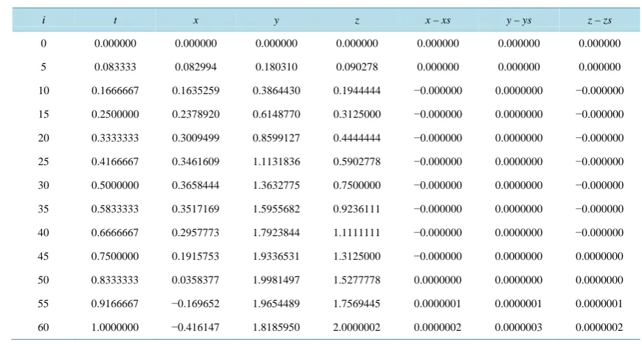
Some results are illustrated inTable 1. (xs, ys and zs are values from the exact solution).

The second problem is a classical example of the DAE problem which is “The pendulum problem”, as ex-pressed in the xy co-ordinate plane as follows:

( )

( ) ( )

( )

( ) ( )

( )

2

( )

2 2

, 0

x t l t x t t y t l t y t g x t y t L



′′ = − ≥



′′ = − − 



+ = _

(8)

where g = 9.8. This problem is an index 2 semi-explicit DAE problem. [3], [10]. Proceeding to solve the prob-lem numerically, we let L = 1, and impose the initial conditions x(0) = 1, y(0) = 0. Using the new variables

1 , 2 , 3 and 4 '

[image:6.595.79.540.96.343.2]

Table 1. Resulting values for x(t), y(t) and z(t) from Algorithm A, and the errors.

i t x y z x – xs y – ys z – zs

0 0.000000 0.000000 0.000000 0.000000 0.000000 0.000000 0.000000

5 0.083333 0.082994 0.180310 0.090278 0.000000 0.000000 0.000000

10 0.1666667 0.1635259 0.3864430 0.1944444 −0.000000 0.0000000 −0.000000

15 0.2500000 0.2378920 0.6148770 0.3125000 −0.000000 0.0000000 −0.000000

20 0.3333333 0.3009499 0.8599127 0.4444444 −0.000000 0.0000000 −0.000000

25 0.4166667 0.3461609 1.1131836 0.5902778 −0.000000 0.0000000 −0.000000

30 0.5000000 0.3658444 1.3632775 0.7500000 −0.000000 0.0000000 −0.000000

35 0.5833333 0.3517169 1.5955682 0.9236111 −0.000000 0.0000000 −0.000000

40 0.6666667 0.2957773 1.7923844 1.1111111 −0.000000 0.0000000 −0.000000

45 0.7500000 0.1915753 1.9336531 1.3125000 −0.000000 0.0000000 0.0000000

50 0.8333333 0.0358377 1.9981497 1.5277778 0.0000000 0.0000000 0.0000000

55 0.9166667 −0.169652 1.9654489 1.7569445 0.0000001 0.0000001 0.0000001

60 1.0000000 −0.416147 1.8185950 2.0000002 0.0000002 0.0000003 0.0000002

1 2 2 1 3 4 4 3 y y y y y y y y g

λ λ ′ =   ′ = − _  ′ = _  ′ = − _{− } initial conditions:

( )

( )

( )

( )

1 2 3 4 0 1 0 0 0 0 0 0 y y y y = = = = (9a) algebraic equation: 2 2

1 3 1 0

y +y − = (9b) If we let x=sinθ, y=– cosθ, substitute in the problem (8) and manipulate some derivatives and algebra, we will obtain the equivalent initial value problem of an ordinary differential equation:

( )

(

( )

)

( )

sin , 0

π 0

2

t g t t

θ θ θ  ′′ = − ≥  

= _ (10)

From (9b) if we differentiate the equation y t1

( )

2+y t3

( )

2=1 twice, we will obtain the equation:

( )

( )

2

( )

2

( )

2 4 2 .

t y t y t gy t

λ = + − (11)

The system (9a) with (11) becomes a pure ODE, since the function λ(t) is expressed in the terms y2

( )

t and

( )

4

y t explicitly.

[image:7.595.85.539.101.362.2]

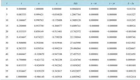
Table 2.Result values for x (t), y (t) and λ (t) from Algorithm B, and the errors.

i t x y λ(t) x – xs y – ys λ – λs

0 0.000000 1.000000 0.000000 0.0066694 0.000000 0.000000 −0.01334

5 0.083333 0.999421 −0.034020 1.2067764 0.000000 0.000000 −0.01327

10 0.166667 0.990763 −0.135608 4.3889120 0.000000 0.000000 −0.01245

15 0.250000 0.953758 −0.300577 9.4089741 −0.000000 −0.000000 −0.00924

20 0.333333 0.858149 −0.513401 15.762372 −0.000000 −0.000000 −0.001840

25 0.416667 0.674223 −0.738528 22.336944 0.000000 0.000000 0.009746

30 0.500000 0.392046 −0.919946 27.443990 0.000000 0.000000 0.021502

35 0.583333 0.039516 −0.999219 29.406564 0.000001 0.000000 0.026667

40 0.666667 −0.320679 −0.947188 27.497515 0.000001 −0.000000 0.021650

45 0.750000 −0.621722 −0.783238 22.424766 −0.000001 0.000001 0.009949

50 0.833333 −0.826959 −0.562262 15.858262 0.000001 −0.000000 −0.001681

55 0.916667 −0.939329 −0.343017 9.4922857 0.000000 −0.000000 −0.009152

60 1.0000000 −0.986140 −0.165918 4.4483962 0.000000 −0.000000 −0.012414

pare to the results from Algorithm B, as shown inTable 2. The value xs, ys and λs are from problem (10). Note that the value of λ(t)'s are at the mid-points t + h/2.

The third problem is an index-2 Hessenberg DAE system with nonlinear differential equations and a nonlinear algebraic equation, as follows:

( )

( )

(

4

( )

1

)

2 1 3

(

) ( )

, 0 1

x t′′ =x t z t − + − t y t ≤ ≤t

( )

2 sin

(

( )

)

( )

(

4

( )

1

)

y t′′ = z t +y t z t −

initial conditions,

( )

0 0,

( )

0 1,

x = y =

( )

0 0,

( )

0 0

x′ = y′ =

algebraic equation

( )

( )

2 2 2 2

x t +t y t =t

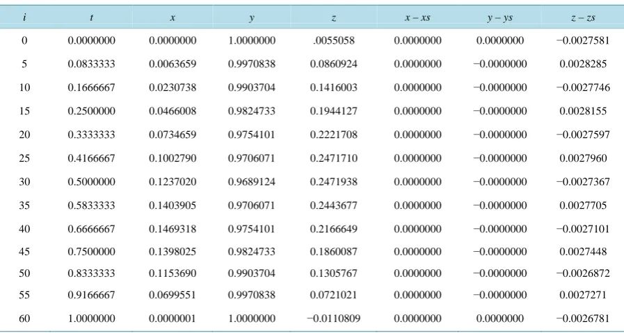
Note that this problem is similar to the first problem, but there is no variable z(t) in the algebraic equation. Using Algorithm B, this problem is solved, and provides a nice result as shown inTable 3. The exact solution is as follows:

( ) (

1

)

z t =t −t

( )

sin

(

( )

)

,

x t =t z t

( )

cos

(

( )

)

.

y t = z t

[image:8.595.89.538.98.338.2]

Table 3. Result values for x (t), y (t) and z (t) from Algorithm A, and the errors.

i t x y z x – xs y – ys z – zs

0 0.0000000 0.0000000 1.0000000 .0055058 0.0000000 0.0000000 −0.0027581

5 0.0833333 0.0063659 0.9970838 0.0860924 0.0000000 −0.0000000 0.0028285

10 0.1666667 0.0230738 0.9903704 0.1416003 0.0000000 −0.0000000 −0.0027746

15 0.2500000 0.0466008 0.9824733 0.1944127 0.0000000 −0.0000000 0.0028155

20 0.3333333 0.0734659 0.9754101 0.2221708 0.0000000 −0.0000000 −0.0027597

25 0.4166667 0.1002790 0.9706071 0.2471710 0.0000000 −0.0000000 0.0027960

30 0.5000000 0.1237020 0.9689124 0.2471938 0.0000000 −0.0000000 −0.0027367

35 0.5833333 0.1403905 0.9706071 0.2443677 0.0000000 −0.0000000 0.0027705

40 0.6666667 0.1469318 0.9754101 0.2166649 0.0000000 −0.0000000 −0.0027101

45 0.7500000 0.1398025 0.9824733 0.1860087 0.0000000 −0.0000000 0.0027448

50 0.8333333 0.1153690 0.9903704 0.1305767 0.0000000 −0.0000000 −0.0026872

55 0.9166667 0.0699551 0.9970838 0.0721021 0.0000000 −0.0000000 0.0027271

60 1.0000000 0.0000001 1.0000000 −0.0110809 0.0000000 0.0000000 −0.0026781

5. Conclusion

The methods are constructed with the objective of solving DAE systems in their original forms. Both algorithms use the Runge-Kutta method as the integrator, and couple this with a method to solve the algebraic systems as-sociated in the problem. The Newton method is used in Algorithm A for index-1 DAE, while in Algorithm B the Newton-Broyden method is needed for an index-2 DAE system. The methods can give approximate solutions for the problem very well, with only small errors. Experiments have also shown that high index DAEs are harder to solve than lower index DAEs.

Acknowledgements

The author would like to thank the referees for their comments. This work was financially supported by the Re-search Grant of Burapha University through National ReRe-search Council of Thailand (Grant No. 35/2556).

References

[1] Ascher, U.M. and Petzold, L.R. (1998) Computer Method for Ordinary Differential Equations and Differential-Alge- braic Equations. Society for Industrial and Applied Mathematics (SIAM), Philadelphia.

http://dx.doi.org/10.1137/1.9781611971392

[2] Brenan, K.E., Campbell, S.L. and Petzold, L.R. (1996) Numerical Solution of Initial-Value Problems in Differential- Algebraic Equations, Revised and Corrected Reprint of 1989 Original, with an Additional Chapter and Additional Ref-erences. Classic in Applied Mathematics, 14. SIAM, Philadelphia.

[3] Campbell, S.L., et al. (2008) Differential-Algebraic Equations. Scholarpedia, 3, 2849. http://dx.doi.org/10.4249/scholarpedia.2849

[4] Rabier, P.J. and Rheinboldt, W.C. (2002) Theoretical and Numerical Analysis of Differential-Algebraic Equations. Hand Book of Numerical Analysis, 8, 183-540. http://dx.doi.org/10.1016/S1570-8659(02)08004-3

[5] Riaza, R. (2008) Differential-Algebraic System: Analytical Espects and Circuit Applications. World Scientific, Singa-pore City.

[6] Hairer, E. and Wanner, G. (1998) Solving Ordinary Differential Equation. II. Stiff and Differential-Algebraic Problems, 2nd Edition, Springer Series in Computational Mathematics, 14. Springer-Verlag, Berlin.

[7] Chompuvised, K. and Dhamacharoen, A. (2011) Solving Boundary Value Problems of Ordinary Differential Equations with Non-Separated Boundary Conditions. Applied Mathematics and Computation, 217, 10355-10360.

[8] Dhamacharoen, A. (2014) An Efficient Hybrid Method for Solving Systems of Nonlinear Equations. Journal of Com-putational and Applied Mathematics, 263, 59-68. http://dx.doi.org/10.1016/j.cam.2013.12.006

[9] Dhamacharoen, A. and Chompuvised, K. (2013) An Efficient Method For Solving Multipoint Equation Boundary Value Problems. World Academy of Science, Engineering and Technology, 7, 329-333.