University of New Orleans University of New Orleans
ScholarWorks@UNO
ScholarWorks@UNO
University of New Orleans Theses and
Dissertations Dissertations and Theses
Summer 8-9-2017
Study of Static and Dynamic Properties of Magnetic
Study of Static and Dynamic Properties of Magnetic
Nanostructures
Nanostructures
Shankar Khanal [email protected]
Follow this and additional works at: https://scholarworks.uno.edu/td
Recommended Citation Recommended Citation
Khanal, Shankar, "Study of Static and Dynamic Properties of Magnetic Nanostructures" (2017). University of New Orleans Theses and Dissertations. 2382.
https://scholarworks.uno.edu/td/2382
This Thesis is protected by copyright and/or related rights. It has been brought to you by ScholarWorks@UNO with permission from the rights-holder(s). You are free to use this Thesis in any way that is permitted by the copyright and related rights legislation that applies to your use. For other uses you need to obtain permission from the rights-holder(s) directly, unless additional rights are indicated by a Creative Commons license in the record and/or on the work itself.
Study of Static and Dynamic Properties of Magnetic Nanostructures
A Dissertation
Submitted to the Graduate Faculty of the University of New Orleans in partial fulfillment of the requirements
for the degree of
Doctor of Philosophy In
Engineering and Applied Science Physics
By Shankar Khanal
B.Sc. Tribhuwan University, 2006 M.Sc. University of New Orleans, 2014
ii
Acknowledgements
My great gratitude goes to Prof. Leonard Spinu for providing me an opportunity to join his research
group. His consistent support regarding academic as well as personal aspects was truly significant.
I am thankful to committee members Dr. Leszek Malkinski, Dr. Weilie Zhou, Dr. John Wiley and Dr.
Damon Smith for their support. Theirs comments and suggestions were substantial to put everything in
context.
Thank you Dr. J M Vargas, Dr. C. Garcia, Dr. C. A. Ross, Dr. R. A. Gallardo for providing the exchange bias
samples and working together as collaborators.
I would like to appreciate the help received from Poncho and Jennifer with all administrative paperwork
during my tenure at AMRI. I would like to thank Harry J. Rees for helping to solve technical problems
with instruments.
I am thankful to our present and past group members: Daniel, Pemba, Jose, Artur, Abhishek, Andrei,
Pratik, Asif, Denny, Nicolas and Ali. I also like to thank Taha, Satish, Rahmat, Zheng, Shuke and all
graduate as well as undergraduate students in AMRI.
It would be impossible to complete sample fabrication and characterization process without having
access to MINT center University of Alabama, Tulane University (CIF microscopy lab), Louisiana State
University (shared instrumentation facility). I would like to thank the people who helped me on these
institutions.
It would be hard to imagine to complete my PhD without funding support from NSF award
ECCS1101798, LASiGMA award No EPS-10003897 and NSF grant No. ECCS – 1546650.
Finally, I would like to acknowledge my thankfulness to all my family members and Love to my wife
iii
Table of Contents
Abstract ... vi
Introduction ... 1
Chapter 1: Overview of Magnetism ... 4
1.1 Introduction ... 4
1.2 Magnetic interaction and energies: ... 5
1.3 Exchange interaction ... 5
1.4 Dipole interaction ... 6
1.5 Magnetic Anisotropy: ... 6
1.5.1 Magneto-crystalline anisotropy: ... 7
1.5.2. Shape anisotropy: ... 8
1.5.3 Magnetostriction and stress anisotropy: ... 10
1.6 Stoner Wohlfarth model ... 10
1.7 Magnetic domain ... 14
1.8 Domain wall ... 15
1.9 Magnetization dynamics ... 19
1.10 Ferromagnetic resonance and high frequency susceptibility ... 20
1.11 Spin wave ... 22
Chapter 2: Sample fabrication and characterization techniques ... 26
iv
2.1.1Design of coplanar waveguide (CPW) ... 26
2.1.2Electron beam lithography (EBL): ... 31
2.3Focus ion beam (FIB): ... 31
2.2 Characterization techniques ... 32
2.2.1 Static characterizations techniques ... 32
2.3.1Vibration sample magnetometer (VSM) ... 33
2.3.2 Magneto-Optic Kerr Effect (MOKE) spectroscopy ... 34
2.3.3Magnetic Force Microscopy (MFM) ... 36
2.4 Dynamic characterization techniques ... 39
2.4.1 Ferromagnetic resonance ... 39
Chapter 3: Exchange bias in (FeNi/IrMn)n multilayer films evaluated by static and dynamic technique. ... 41
3.1Introduction to exchange bias effect ... 41
3.2 Sample preparation and characterization techniques: ... 44
3.3Static experimental results ... 45
3.4Dynamic experimental results: ... 50
3.5Angular dependent FORC and FMR of exchange-biased multilayer systems: ... 57
3.6 AFORC diagrams and profiles: ... 58
3.7Angular ferromagnetic resonance study (AFMR) at X-band: ... 63
Chapter 4: Static and dynamic properties surface of modulated structure ... 69
v
4.2 Sample preparation techniques ... 70
4.3 a varied systems ... 71
4.4 Micromagnetic Simulation ... 77
4.5 b varied systems:... 81
4.6 Results and discussions ... 82
Chapter 5: Static and dynamic study of shape modulated structures... 86
5.1 Introduction ... 86
5.2 Static and dynamic study of dumbbell structure ... 87
5.3 Sample preparation ... 87
5.4 Experimental and static micromangetic results... 90
5.5 Experimental dynamic results: ... 94
5.4 Micromagnetic simulated results for ferromagnetic resonance spectra. ... 96
Conclusion and future work ... 102
References ... 105
vi
Abstract
Magnetic materials are one of the most interesting and promising class of materials for technological
applications [1]. Among them, patterned ferromagnetic systems have an important role especially in the
prospect of high density data storage [2], domain wall logic devices [3] and magnetic memory [4, 5].
Coupled systems of ferromagnetic and antiferromagnetic materials have been implemented to design
sensors such as giant magnetoresistance (GMR) [6-8] and tunnel magnetoresistance (TMR) [9, 10].
Ferromagnetic nanoparticles have been used for the drug targeting, cancer therapy, Magnetic
Resonance Imaging (MRI) and many more applications [11, 12]. In addition, more recently, significant
attention has been paid to the exploration of the dynamic properties of magnetic materials in the GHz
range and use them for technological applications such as microwave filters, signal processing, phase
shifter, nonreciprocal microwave devices, spin wave guide, high frequency memory, logic elements
[13-19]
Boundary conditions, interactions between individual entities, and lateral confinement of magnetic
charges generate diverse magnetic properties especially at nanoscale length [20, 21]. The variation of
magnetic properties are quite different when the size of the magnetic structure is smaller or comparable
with the magnetic characteristic length such as mean free path of electron, width of domain wall and
even the spin diffusion length [22-24].
In this study, we have considered different magnetic systems with at least one dimension in the
nanometer scale, i.e. magnetic nanostructures. Firstly, the multilayers of coupled ferromagnetic and
antiferromagnetic system have been considered to evaluate the exchange bias anisotropy. [FeNi/IrMn]n
multilayer systems with different thicknesses of ferromagnetic layer and exchange bias strength were
studied. Their static and dynamic properties were revealed through Vibrating Sample Magnetometry
vii
first order reversal curve (AFORC) and ferromagnetic resonance (AFMR) were performed to learn the
intrinsic exchange bias distribution. Secondly, patterned periodic magnetic structures, i.e. magnonic
crystals, were synthesized to understand the magnetization dynamics in confined geometry. Surface
modulated thin films with different periodicity, dumbbell-shaped structures with variable size and three
dimensional magnonic crystals have been studied using both static and dynamic measurement
techniques. Micromagnetic simulations were performed to understand and explain the experimental
results.
Keywords: magnetic nanostructures, ferromagnetic resonance, exchange bias, coplanar waveguide,
1
Introduction
The most fascinating aspect of magnetic materials is that their properties are strongly dependent on the
physical shape, size, the distance between them as well as their symmetry [25, 26]. Thin films, patterned
structures, free nanoparticles and now three dimensional magnetic structures have attracted incredible
attention in scientific community. Control of magnetization with external magnetic field, temperature,
spin current and pressure make magnetic systems more interesting regarding both fundamental as well
as technological application [27]. Development in cloud computing to improve data storage has been
pushed to a different level because of the better understanding of magnetism at nanoscale [28].
Understanding domain, domain walls, and their dynamics are always fascinating as sensors to read and
write data [29]. In dynamic aspect, spin wave dynamics have been emerging in confined magnetic
nanostructures with the possibility of tuning them in wide range of frequency, so called magnonics
[30-32]. Magnonics for future data storage and logic has been already realized [31]. Magnonic crystal, which
has alternative properties within the system, can be achieved without complicated compositional
changes.
In addition, magnetic multilayer systems are the most promising asset in many technological
perspectives [33-35]. Among them, exchange bias, which exists at the interface between ferromagnetic
and antiferromagnetic layers, has been already implemented as a sensor to read and write data in
magnetic memory. The superparamagnetic effects, especially occurring for nanometer scale magnetic
materials, can be controlled by considering the coupling of antiferromagnetic material with magnetic
nanostructure [36].
In this thesis, different aspects of magnetism have been revealed. Coupling scheme between
2
structures have been fabricated and characterized with different techniques. The outline of the thesis
will be presented in the following.
Chapter 1 presents on overview of magnetism concepts that will be used in the subsequent chapters.
The different scientific terms and energy terms involved in magnetic materials will be discussed. The
magnetic switching in the static regime will be described using the Stoner-Wohlfarth model. The
existence of magnetic domain in ferromagnetic materials, domain walls and their dynamics will be
presented. Magnetization switching in the dynamic regime will be explained using the Landau-
Lifshitz-Gilbert (LLG) equation. Ferromagnetic resonance phenomenon that will used to characterize the
dynamic properties of studied magnetic nanostructures will be presented. Theory of spin wave dynamics
in magnetic thin film is also discussed.
Chapter 2 describes Sample Fabrication and Characterization Techniques. Fabrication techniques such as
photolithography, electron beam lithography, focused ion beam, sputtering, and liftoff have been
discussed. Design of micrometer size coplanar waveguide (CPW) and fabrication of magnetic structures
exactly on the top has been achieved. Static and dynamic characterizations have been performed using
different characterization techniques. For example, the static case, Vibrating Sample Magnetometer
(VSM), First Order Reversal Curve (FORC), Magneto-optical Kerr Effect (MOKE) and magnetic force
microscopy (MFM) have been reviewed. In dynamic regime, the X-band ferromagnetic resonance at 9.8
GHz and broad band vector network analyzer ferromagnetic resonance (VNA-FMR) technique have been
presented.
Chapter 3 is about the Exchange bias in (FeNi/IrMn)n multilayer films evaluated by static and dynamic
techniques. We studied the coupled ferromagnetic and anti-ferromagnetic system by varying the
thickness of ferromagnetic layer. The static and dynamic properties of these coupled systems have been
3
properties have been performed using angular FORC (AFORC) technique. The angular dependent
dynamic properties have been studied using angular FMR. Finally, results from both techniques have
been compared.
In chapter 4, static and dynamic properties surface modulated structures were studied. This chapter
presents the study of several configuration of one dimensional magnonic crystals. Surface modulated
structures were fabricated using a combination of different techniques. The periodicity of modulated
region was varied to understand their effect on the statics and dynamic properties. Angular variation of
Major Hysteresis Loops was measured to study the static properties. The angular dependence FMR was
used to reveal the field and frequency dependent dynamic properties. The experimental results have
been explained and verified using micromagnetic simulation.
Static and dynamic study of shape modulated structures as well as conclusion and prospective of future
work have been presented in chapter 5. The hybrid structures (dumbbell) of wire and dot have been
considered to evaluate the static and dynamic properties. The size of the dots has been varied to
understand static and dynamic magnetization. The switching of magnetization in confined and restricted
geometry has been studied in static case. In terms of dynamics, excitation and propagation of spin
4
Chapter 1: Overview of Magnetism
1.1 Introduction
In this chapter, it will be presented the fundamental concepts and scientific terms which will facilitate to
understand the following chapters.
Microscopically, magnetism originates from the motion of electrons around nucleus. There are two
types of motion of an electron. The first is that electron revolves around the nucleus and generates
orbital angular momentum. Similarly, the second is the electron spins around its own axis and generates
spin angular momentum. Finally, the total angular momentum is the sum of these two momenta.
However, classically, magnetic moment (𝜇), which is considered as fundamental unit of magnetism, can
be explained by comparing angular momentum of electron with the current in a loop. For example, if
current (I) is flowing in a circular wire and area enclosed by the wire is A, the magnetic moment
associated with that moving electron can be expressed as
μ = I. A (1.1)
Where, A is the area enclosed by circle.
Magnetic moment can now be expressed in terms of angular momentum (L = m v r) by simply
substituting value of current (I=e/t) and A in equation 1.1.
μ = ( e
2m) L (1.2)
Substituting γ = e/2m, magnetic moment finally can be written as;
μ = −γ L (1.3)
where, 𝛾 is gyromagnetic ratio.
5
d𝛍 dt = γ
d𝐋 dt = γτ
(1.4)
In presence of external magnetic field (H), the equation of motion for the magnetic moment is
d𝛍
dt = γ 𝛍×𝐇
(1.5)
Finally, total energy of magnetic moment on external magnetic field can be expressed as
E = −μ0𝛍. 𝐇 (1.6)
1.2 Magnetic interaction and energies:
A unique property of magnetic materials is that they interact with other magnetic materials, especially
ferromagnetic materials. Magnetic moments in ferromagnetic materials align in certain orientation even
in the absence of external field and have spontaneous magnetization. The interaction can be between
neighboring magnetic moments or with external magnetic field. In addition, interaction may be classical
or quantum in origin. The main interactions, especially in ferromagnetic materials, are dipole and
exchange interactions. In the following section, they will be described in brief.
1.3 Exchange interaction
Exchange interaction, which is quantum in origin, initiates as a result of quantum mechanical interaction
between electrons. It is important to mention that depending on the orientation of a spin with respect
to the neighboring one, the materials are classified as ferromagnetic, anti-ferromagnetic and
ferromagnetic. Let us consider the exchange interaction between two electrons with spin S1 and S2 . The
Hamiltonian because of exchange interaction for two electrons system is written as,
𝑯𝑒𝑥= −2𝐽12𝑺1. 𝑺2 (1.7)
6
𝐽12= ∬ Ψ1 (𝑟1)Ψ2 (𝑟2)𝐻𝑒𝑥 Ψ1 (𝑟2)Ψ2 (𝑟1) 𝑑3𝑟1𝑑3𝑟2 (1.8)
It is important to mention that although the exchange interaction is very strong, it decays exponentially
with space. However, this interaction is strong enough to keep neighboring spin align together. Finally,
Positive value of J corresponds to the parallel alignment of spin and results ferromagnetic ordering.
Negative value of J causes the antiparallel orientation of spins and leads anti-ferromagnetism.
1.4 Dipole interaction
Let us consider two magnetic dipoles µ1 and µ2 which are separated by distance r. The dipolar
interaction energy, from electromagnetism, can be expressed as [37]
Edipole = μ0/4πr3[𝛍𝟏. 𝛍𝟐−
3
r3(𝛍𝟏. 𝐫)(𝛍𝟐. 𝐫)]
(1.9)
Where, µ0 is permeability of free space. From above equation it can be clearly observed that dipolar
energy depends on the third order of the distance between dipoles. Since the dipolar interaction exists
at long range, it has significant contribution on demagnetization field as well as for long wavelength spin
waves.
1.5 Magnetic Anisotropy:
Magnetic materials are anisotropic, i.e., their static and dynamic properties are strongly dependent on
the direction of the applied field. In terms of origin, some anisotropies are intrinsic in nature, such as
magneto-crystalline, and some are extrinsic, for example shape anisotropy. Tuning magnetic properties
by manipulating these anisotropies is critical in fundamental as well as technological applications. Most
7
1.5.1 Magneto-crystalline anisotropy:
Magneto-crystalline anisotropy is induced due to spin-orbit interaction in magnetic materials[38]. Spin-
spin coupling assists to keep spins either parallel or anti-parallel and it simply depends on the angle
between them. Hence, it does not necessarily depend on the crystal axis, and spin-spin interaction does
not help to induce magneto-crystalline anisotropy[38]. In contrast, the coupling of orbit with lattice is
strong. This strong quenching of orbital magnetic moment with the lattice needs a much stronger field
to breakdown coupling and results magneto-crystalline anisotropy.
Generally, the direction of easy axis is the direction of spontaneous magnetization in the demagnetized
state. External work is needed to rotate the magnetization from easy axis to any other orientations.
Depending on the type of crystals, there would be cubic or hexagonal magneto-crystalline anisotropy.
For cubic crystal, if magnetization (Ms) orients with cosine angle α1, α2 and α3 with crystal axis a, b, and
c respectively, the cubic anisotropy can be expressed as [38],
E = K0 + K1(α12 α22+ α22α32+ α32α12) + K2(α12 α2 2α32)+…….. (1.10)
Where, K0, K1 and K2 are anisotropy constants, and they depend on temperature as well as type of
material.
In case of hexagonal materials, for example cobalt, the basal plane is equally magnetically hard. Thus,
anisotropy energy depends on the angle between Ms and c axis of the crystal. For example, if θ is the
angle between Ms and c axis, the anisotropy energy can be expressed as
E = K0 + K1 sin2Ѳ + K2 sin4Ѳ + ⋯ (1.11)
8
The hexagonal crystal structure of cobalt and the magnetization vs field at different crystalline axes are
presented in figure 1.1. When the angle θ is zero, there will be minimum energy thus the c-axis is the
easy axis of magnetization. The dependence of magnetization with the magnetic field for two different
axis of crystal for cobalt is presented in figure 1.1 [b].
1.5.2. Shape anisotropy:
The orientation of spontaneous magnetization in ferromagnetic materials also depends on its own
shape. For example, spherical shape samples are isotropic. In contrast, if the sample is not spherical, it is
easy to magnetize in one orientation than other. If we consider a long wire, it is easy to magnetize along
the length of wire rather than perpendicular to it. The demagnetization field opposes the external
applied field and reduce effective field. Generally, shape anisotropy is expressed in terms of
9
Ems=
1 8π∫ Hd
2dv (1.12)
The magneto-static energy in vector form is written as
E = − 1
2 𝐇𝐝 . 𝐌
(1.13)
The negative sign is for the opposite direction of Hd with M.
Now let us consider a prolate spheroid to calculate the magneto-static energy. The semi-minor and
major axis are represented by a and c respectively in figure 1.2.
If we consider the component of magnetization along the c-axis, the magneto-static energy can be
expressed as,
Ems=
1
2 [(M cosθ)
2N
c+ (M sinθ)2Na (1.14)
Na and Nc are the demagnetization factors along the a and c-axis. Substituting the cosθ with sinθ,
equation 1.18 becomes,
Ems=
1 2 M
2N c+
1
2 (Na − Nc)𝑀
2 (sinθ)2 (1.15)
10
1.5.3 Magnetostriction and stress anisotropy:
When external magnetic field is applied to ferromagnetic materials, the dimension of these materials
changes during magnetization process. The resulting strain is called magnetostriction (λ) [39]. In case of
one dimensional structure, it can be expressed as[40],
λ = dl/l (1.16)
Where, dl is the change on length (l).
1.6 Stoner Wohlfarth model
Stoner Wohlfarth model explains the magnetization reversal curve for single domain specimen with
uniaxial anisotropy[41]. The uniaxial anisotropy might be because of shape anisotropy or
magneto-crystalline anisotropy or both. Let us consider the ellipsoidal shaped single domain specimen as in figure
11
If θ is the angle between the magnetization (Ms) and easy axis, anisotropy energy can be expressed
as[40]
Ean= K sin2θ
The misalignment of easy axis and magnetization induce torque and it is written as,
τan= −
dEan
dθ
= −2K sinθ cos θ
If external field is applied (H) as shown in figure1.4, torque produce due the external field is
𝛕H= μ0 𝐌𝐬×𝐇
= μ0 HMs sinφ
12
Where, ϕ is angle between magnetization and field direction.
At equilibrium condition, sum of torques due to and external field and anisotropy is zero i.e.
τH+ τan= 0
μ0 HMs sin (α − θ) −2 K sinθcosθ= 0
If Hk is the field strength to rotate the magnetization from easy axis, which is 90 degree with applied
field to the field direction, then the anisotropy field can be expressed as
Hk = 2K/μ0Ms (1.17)
If the applied field is perpendicular to the anisotropy field it creates reversible changes of magnetization
as in figure 1.4(b)
However, for magnetic field and anisotropy field are parallel, the magnetization switching is irreversible
if applied field is less then 2K/μ0Ms as in figure 1.5
13
For the applied magnetic field at arbitrary direction with the anisotropy axis, both the reversible and
irreversible components of magnetization contribute on MHL. MHL for a spherical single domain particle
when the external magnetic field is at 450 with the anisotropy field is presented figure 1.6.
Figure 1.5: (a) magnetic field parallel to easy axis with anisotropy field Hk (b) MHL for case corresponds to (a)
14
Despite the wide application of Stoner – Wohlfarth model, there are limitations to apply this model in
many practical aspects. The reasons for that are this model does not consider the effect of interaction
between the particles, temperature dependence magnetization and multi-domain magnetic systems.
1.7 Magnetic domain
Magnetic moments, in ferromagnetic materials, are aligned parallel within small volume is called
magnetic domain. The orientation of the magnetic moments in a domain will be different from the
neighboring one. The boundary wall between two domains is called domain wall. Depending on the
nature of orientation of spins in domains walls, domain wall are classified in different categories.
Generally Bloch wall presents on the bulk materials and Neel wall on the thin samples. In addition, there
is very interesting phenomena for the formation of domain wall especially in ferromagnetic materials.
The systematic of the domains formation will be discussed here considering a bar magnet as in figure
1.7.
15
When external magnetic field is applied along a bar magnet as in figure 1.7[a], the magnet is saturated
and the magnetic surface charges appear at the edge of the magnet. There will be a demagnetization
field associate with these surface charges which essentially reduce the effective magnetic field of
sample. Energy associate with these surface charges is called magneto-static energy. One way to reduce
magneto-static energy is to divide the single domain magnet in multi-domain as in figure1.7 [b] and [c].
When magnetic moment within a bar magnet oriented in opposite direction, the distance between the
positive and negative charge decrease and consequently the spatial extend of the demagnetization field
also decrease. However, one thing we need to keep in mind is that this process does not go infinitely.
The reason is that there will be a domain wall between two domains and the energy is required to
create and maintain domain wall. When the magneto-static energy is equal with the energy required to
maintain domain wall, the equilibrium will be reached and splitting of domain stops.
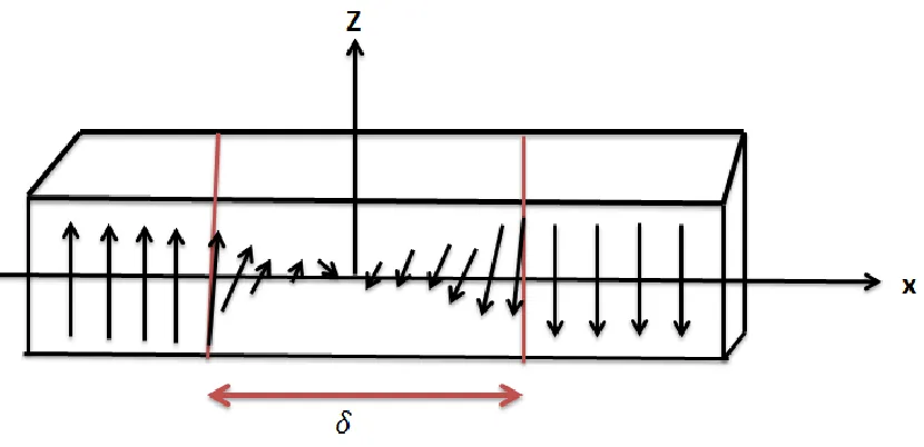
1.8 Domain wall
As discuss earlier, the domain wall is an interface between the two domains where spontaneous
magnetization are at different orientations. The change of magnetization in the interface between two
domains is not abrupt. As presented in figure 1.9, the orientation of the magnetic moment might be
1800 (Bloch wall) or 900 (Neel wall) or any other depending on the geometry as well as composition of
specimen. In the following, we will calculate the domain wall width for Bloch type domain wall which is
16
Let us consider two closest spins S1 and S2, the exchange energy between them can be expressed as [40]
Eex= −2 J12 S1 . S2= −2JS2cosθ
This means that the exchange energy depend on the angle between two spins. For example, if the angle
between two spin is π, there will be maximum exchange energy. Let us consider a wall with N lattice
spacing so angle between two neighboring lattices is
𝜃 = 𝜋 𝑁
The exchange energy difference, when first spin at zero degree orientation and second with small theta,
is
∆𝐸𝑒𝑥= 𝐸𝑒𝑥− 𝐸𝑒𝑥𝜃=0
= −2𝐽𝑆2 𝑐𝑜𝑠𝜃 + 2𝐽 𝑆2
≈ 2𝐽𝑆2[1 − 1 + 𝜃2]
17
≈ 2𝐽𝑆2𝜋
2
𝑁2
Total energy for N spin is expressed as,
𝐸𝑒𝑥𝑡𝑜𝑡𝑎𝑙 = 𝑁𝐽𝑆2
𝜋2
𝑁2 = 𝐽𝑆 2𝜋2
𝑁
If a is the lattice constant, the exchange energy per unit area is
𝜎𝑒𝑥 = 𝐽𝑆2 𝜋
2
𝑁𝑎2
(1.15)
Thus if N→∞, σex → 0, it means wide domain wall is preferred for minimum energy, which means the
spin will be randomly oriented. However in case of ferromagnetic materials, this does not occur because
the magnetic anisotropy energy increases when the spins are randomly oriented. Thus, width of the
domain wall is determined by the balance between the exchange and magnetic anisotropy energies. To
calculate the anisotropy energy, let θ is the angle between the easy axis and the magnetic dipole, the
magnetic anisotropy could be expressed as[40],
𝐸𝑎𝑛𝑖 ≈ 𝐾𝑢 𝑠𝑖𝑛2𝜃
If there are N lattice along the wall, the total energy is
𝐸𝑎𝑛𝑖𝑡𝑜𝑡𝑎𝑙= ∑ 𝐾𝑢 𝑁
𝑖=1
18
Since total anisotropy constant is per unit volume, the anisotropy energy density per unit area is
𝜎𝑎𝑛𝑖=
𝑁𝐾𝑢𝑎
2
The total energy associate with Bloch domain wall per unit area can be expressed as
𝜎 = 𝜎𝑒𝑥+ 𝜎𝑎𝑛𝑖
= 𝐽𝑆2 𝜋 2
𝑁𝑎2+
𝑁𝐾𝑢
2
The number of lattice spacing can be derived by minimizing the energy density of wall
𝑑𝜎 𝑑𝑁= −
𝐽𝑆2𝜋2 𝑁2𝑎2 +
𝐾𝑢𝑎
2 = 0
⇒ 𝑁 = 𝜋S√ 2𝐽 𝐾𝑢𝑎3
Substituting this value in above equation, the domain wall width can be expressed as,
𝜎𝑒𝑥= 𝐽𝑆2 𝜋
2
𝑁𝑎2
(1.16)
The equation (1.16) clearly suggests that the width of the domain wall depends on the exchange integral
and anisotropy constant. The domain wall width increases when the exchange integral increases and
decrease when the anisotropy constant increase. The competition between these two energies
19
1.9 Magnetization dynamics
So far we have discussed static magnetic properties of magnetic specimens. In the following, we will be
discussing about the dynamics of magnetic moments especially in presence of external magnetic field.
For this, let us consider external magnetic field is applied in ferromagnetic material which forces the
magnetic moments to align along the field direction and precess. We have already discussed the torque
on the magnetic moment (μ) due to the external field. Again, it can be expressed as
𝛕 = μ0𝛍×𝐇
Where μ0 represents the magnetic permeability in free space. The torque causes the precession of
magnetic moments with frequency ωL called Larmor frequency. Mathematically it can be expressed as
ωL = μ0γH
Where, γ is gyromagnetic ratio.
The time dependence of the magnetization in presence of external magnetic field can be written as[42]
d𝐌
dt = −γ 𝐌×𝐇
(1.17)
This is the Landau- Lifshitz equation. This equation explains the magnetization dynamic for the system
with uniform magnetization. To realize this dynamic motion practically, if we consider one end of
magnetization fastened and other kept free, it moves on the surface of sphere and this kind of motion is
called precession motion. For the case of cylindrical symmetry, magnetization moves in circle and more
complicated on others configuration.
In reality, the precession of spin dose not last forever. If external magnetic field is turned off, damping of
the oscillation of magnetization amplitude takes place due to the dissipation of the energy. The energy
20
consider this effect, Gilbert introduced an extra term to equation of motion of magnetization (equation
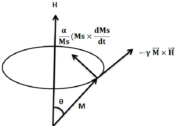
(1.27)). Now the complete equation of motion for the magnetization can be written as[42],
d𝐌
dt = −γ 𝐌×𝐇 + α Ms(𝐌s×
d𝐌s dt )
(1.18)
This equation is Landau-Lifshitz-Gilbert (LLG) equation where α is Gilbert damping parameter. The
systematic of precession and damping of magnetization is presented in figure 1.9. First term in equation
(1.28) contributes for precession and the second term for the damping of magnetization.
1.10 Ferromagnetic resonance and high frequency susceptibility
Ferromagnetic resonance (FMR) is a firmly established experimental technique to determine not only
susceptibility at high frequency but also for anisotropies in magnetic materials [43]. There are two
established approach to do FMR experiment. The first approach is that the microwave with fixed
21
microwave frequency is swept at constant external magnetic field. The most important aspect of FMR
technique is that it allows investigating the ground states of ferromagnetic specimen without
perturbation[44]. The low energy excitation of microwave field allows for it.
The spin dynamic, which occurs at nanosecond time scale, is extremely difficult to observe. For that
reason, it is easy to explain dynamic of spin in frequency domain. In the following, we will be discussing
about how FMR technique can be implemented to get information about magnetic susceptibility at high
frequency.
Let us consider an infinitely large ferromagnetic specimen and external magnetic field(𝐇 = H0. 𝒆𝒛) is
applied along the Z- direction. If the sample is excited with the time dependent microwave field in x-y
plane, i.e.hrf(𝑡) = (hx , hy, 0). 𝑒−𝑖𝜔𝑡, time varying magnetization along the Z-direction the can be
expressed as𝐌 = M𝑠 𝐞𝐳+ 𝐦 𝑒−𝑖𝜔𝑡. If the microwave field and dynamic components of magnetization
are small, we can neglect the product of these two terms which leads the LLG equation as [44]
d𝐦
dt = γ(𝐇0×𝐦rf+ 𝐡𝐫𝐟×𝐌S) + α Ms
𝐌×d𝐦rf dt
≈ 𝛾 𝐞𝐳×(𝐵0𝐦𝑟𝑓− 𝜇0𝑀𝑠𝐡𝑟𝑓) + 𝛼𝑒⃗𝑧×𝐦̇𝑟𝑓
If we consider the ac components of magnetization and magnetic field, the above equation can be
expressed as,
−iωmx+ (γB0− iωα)my= γMsμ0hy
−iωmy− (γB0− iωα)mx= −γMsμ0hx
22
The solution of the above equations can be expressed in terms of polder’s susceptibility tensor which
relates the dynamic magnetization with RF magnetic field [44].
𝐦𝑟𝑓= 𝜒𝐡𝑟𝑓= (
𝜒𝐿 −𝑖𝜒𝑇 0
𝑖𝜒𝑇 𝜒𝐿 0
0 0 0
) ( ℎ𝑥
ℎ𝑦
ℎ𝑧
)
Where 𝜒𝐿=
(𝜔0−𝑖𝜔𝛼) 𝜔𝑀
(𝜔0−𝑖𝜔𝛼)2 and 𝜒𝑇 =
𝜔𝜔𝑀
(𝜔0−𝑖𝜔𝛼)2−𝜔2 are longitudinal and transverse susceptibility
respectively.
And 𝜔0 = 𝛾𝐵0 and 𝜔𝑀= 𝛾𝜇0𝑀𝑆
From above equation it is clearly observed that when α≠0, the susceptibility will not be zero and it gives
non- zero complex susceptibility. In this case, the microwave power will be absorbed by the sample and
mathematically the average power absorbed within sample is
𝑃 =𝜇0 2 𝜔 𝜒𝐿
,,(ℎ 𝑟𝑓 𝜒
)2𝑉
(1.19)
Here V is the volume of specimen and the magnetization is restricted only on X-direction.
1.11 Spin wave
LLG equation describes the magnetization dynamic of homogenously magnetized specimen using
macro-spin approximation. However, in reality, it is extremely hard to realize a specimen with uniform
magnetization because of the thermal fluctuation as well as edge effects on ferromagnetic specimens.
For example, at absolute zero temperature, magnetic moments of ferromagnetic materials are perfectly
aligned but when the temperature reach at Curie temperature the magnetization is completely vanish.
Bloch introduced the temperature dependence of the magnetic moment by stating that the low
temperature dependence excitation of magnetic moment creates wave called spin wave[45]. In fact, the
23
electromagnetic wave or even heat [46]. Heller and Kramers explained the spin wave in terms of the
precessing spins[47]. In ground state, there will be the interaction between the nearby spin which give
rise to the parallel arrangement of them. However, if the external perturbation is applied on the system,
the spins will start to precess with slightly different phase with the neighboring spin and there will be
phase difference which ultimately results the wave like behavior. As shown in figure 1.10 [a], where all
spin precess in phase with infinite wavelength which means that the wave vector (k) is zero. In figure
1.10[b], spins prcecess out of phase with certain wave vector and behave as wave called spin wave.
The wavelengths of the excited spin wave are determined by two factors. For long wavelength, there
will be dipolar dominated interaction and for short wave length there will be the exchange dominated
interaction between spins [48, 49].In addition, there are three main types of spin waves especially in
thin films samples. For a given structure, they are classified by propagation direction of the spin wave
with respect to the external applied field. In the following, we will be discussing about these three types
of modes.
24
Forward volume magneto-static spin wave (FVMSW): FVMSW is excited when the sample is magnetized
in the perpendicular direction with respect to the direction of propagation of spin wave. Dispersion
relation for this configuration can be expressed as [50]
fFVMSW= fH√(fH+ fM(1 −
1 − exp (−kdo)
kdo )
(1.20)
Where fM=4πγM0 and fH=γH0. M0 and do are saturation magnetization and thickness of film respectively.
Similarly, when the sample is magnetized in plane, there exists two types of spin wave and they are
named as backward volume magnetostatic waves (BVMSW) and magnetostatic surface spin waves
(MSSW).
For BVMSW, the propagation of spin wave occurs along the magnetization direction and the dispersion
relation can be expressed as [50]
fBVMSW = fH√(fH+ fM
1 − exp (−kdo)
kdo )
(1.21)
Finally, MSSW generally localized on one surface of thin films. The amplitude of precession is
exponential in nature with the minimum on one surface and maximum on next one. The dispersion
relation for MSSW wave could be expressed as [50]
fBVMSW = fH√(fH+ fM
1 − exp (−kdo)
kdo )
25
The systematic of the direction of propagation of spin wave and magnetization for all configurations is
presented in figure 1.11.
26
Chapter 2: Sample fabrication and characterization techniques
In this chapter, various sample fabrication and characterization techniques will be discussed. In terms of
fabrication techniques; different state of the art techniques have been used. For example,
photolithography, electrons beam lithography, sputtering, lift-off and focus ion beam (FIB). In terms of
characterization methods, several advanced scientific instruments such as Vibrating Sample
Magnetometer (VSM), Magneto Optical Kerr Effect (MOKE), Atomic force microscopy (AFM), Magnetic
force microscopy (MFM) and broadband ferromagnetic resonance (FMR) techniques have been
implemented. In the following sections, all techniques that had been implemented will be discussed
briefly.
2.1Sample fabrication techniques
2.1.1Design of coplanar waveguide (CPW)
The high frequency characterization of almost all samples was carried out using the VNA-FMR
technique. The first step in experimental procedure was to design ideally loss-less CPW. Two types of
CPWs have been fabricated to study the magnetic systems.
The first type of CPW was fabricated to study the thin films samples which were bigger in size and had
strong magnetic signals. Before fabrication of CPW, the CST MWS STUDIO software was used to
determine the shape, size and dimension of CPW and to achieve characteristic impedance of 50 Ohm. It
has been a well-established technique to use dielectric material and conductor to fabricate lossless
transmission lines. Slab of Rogers with gold on both sides were used to fabricate the CPW. Vias from top
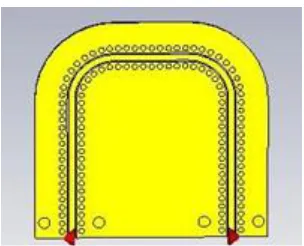
to bottom were created to get uniform electric and magnetic field on the signal line of CPW. The typical
structure of CPW which was used in this study is presented in figure 2.1. The red arrow at the ends
27
Scattering parameters (S-Parameters) are the most important parameters to consider for
characterization of microwave devices. In the process of characterization of magnetic samples, we
tracked these parameters as a function of magnetic field and microwave frequency. In the following, we
will be discussing about S-parameters and express them mathematically
.
The uses of current and voltage concept on a circuit, where hundreds of components (such as resistor,
capacitor and inductor) are involved, are rather complicate [51]. The concept of S-parameter allows us
to get complicated information in a simple way like as a black box. For microwave devices, it is
important to consider that the ports at the end of the circuit’s components are connected with each
other. Transmission and reflection of microwave signal takes place when signal go through the different
ports. Generally the amplitude of these signal are considered to express S-parameter mathematically. In
addition, since S-parameters are complex in nature, which allows us to get information about also the
phase of the signal along the circuit. For N port system, there are N2 S-parameters and we will express
them mathematically in the following.
28
For simplicity, let us consider a two port device. a1 and b1 are the amplitude of incident wave and
reflected wave at port 1 and 2 respectively and a2, b2 are for port 2 as in figure2.2. If the ports are
terminated with the characteristic impedance, the S-parameters are defined as[51],
𝑆11=
𝑏1 𝑎1
𝑆12=
𝑏1 𝑎2
𝑆21=
𝑏2 𝑎1
𝑆22=
𝑏2 𝑎2
We can also express the relation between amplitude of signal and S- parameters in matrix form,
(𝑏1 𝑏2) = (
𝑆11 𝑆12
𝑆21 𝑆22) (
𝑎1 𝑎2)
For lossless transmission lines, it is most important to have characteristic impedance on each port of
components of a device. The simulated normalized impedance of CPW is presented in figure 2.3. The
29
characterized impedance was achieved and pink line represents the variation of impedance with
frequency. The CPW with ideal impedance of 50 Ohm was fabricated.
Now we will be discussing about the second type of CPWs that were fabricated and used to study the
magnetization dynamic of magnetic nanostructure. CPW, which is bigger in size, has lower sensitivity for
smaller amount of sample because the radiation loss is proportional to the volume of CPW[52]. To
overcome this challenge, it is important to fabricate smaller CPW in size. Creating nanostructure directly
on the top of signal line does not only increase sensitivity but it also reduce the fabrication cost of
sample especially using electron beam lithography.
Before fabrication of CPW, the shape, size, structure and materials for CPW was designed using CST
microwave studio. The standard photolithography, sputtering and lift-off process was used to fabricate
30
fabrication of CPW is depicted systematically which involves multiple steps. Similarly in figure 4 [b], the
typical SEM image of final product of CPW is depicted. In brief, the following procedure was used to
fabricate CPW. The positive photoresist was coated on clean silicon substrate using spin coating
technique. Then, it was baked on a hot plate at temperature 1100 C for 1 minute. After that the
substrate was covered with the photomask and exposed with the UV light for 2 minutes. Then it was
developed with the developer. Cr (5 nm)/Cu (150 nm)/Pt (10nm) were deposited with the help of
sputtering technique. Finally lift-off technique was used to achieve CPW with characteristic impedance
of 50 Ohm and the final product is depicted on [b] figure 2.4.
31
2.1.2Electron beam lithography (EBL):
EBL is a state-of- art technique to fabricate especially nanostructures materials[53]. This technique offer
high resolution to produce nanostructures compare to photo-lithography process. Short wavelength of
electron beam overcomes the diffraction effects which especially exist with UV light and ultimately
allows creating structures which is impossible by using photolithography technique. Although the
process that EBL technique works is similar to the photolithography process, the fundamental difference
is that coherent electron beam is used to write pattern in EBL technique whereas UV light is used for the
photolithography process. The resolution up to few nanometers has been achieved using e-beam
lithography technique.
In the following, we will be discussing about the electron beam lithography process in detail. Firstly,
since we were preparing sample on the top of signal line of CPW, the first step was to fabricate CPW.
Substrate, with CPW on it, was coated with 950 Poly-methyl-Methacrylate (PMMA) positive resist. Spin
coater at speed of 4000 rpm was used to distribute resist layer homogenously all over the substrate. The
sample was then baked for 80 second at temperature of 1300 C. The pattern which we would like to
fabricate was designed using AutoCAD software and loaded to the NPGS software. Working distance of
9mm was used on the writing process. The electron beam current of 20 pico-amperes was used to
achieve high resolution patterns. When the writing process completed, resist was developed by using
solution of Methyl-isobutyl-ketone (MIBK) and isopropyl alcohol in 3:1 ratio for 60 second. Finally,
deposition and liftoff process was used to fabricate sample with desired shape and size on the top of
signal line of CPW.
2.3Focus ion beam (FIB):
FIB is an advance technique that has been widely used in semiconductor industry, biology and materials
32
different. In a FIB system, beam of focused ions are used instead of an electron beam as in SEM. The
Quanta 3D DualBeam FEG, which was combined with FIB, was used to fabricate samples. Focused Ga ion
beam was used to etch surface of thin film and to fabricate the periodic pattern structure in the form of
grooves[58]. The samples with high resolution were achieved. During etching process, beam current 1.5
pico-ampere was used. The etching time was kept constant to achieve ideally the constant etched
thickness for all samples. A sample fabricated by etching the material from the surface of Permalloy’s
thin film to produce one dimensional groove and SEM image is presented in figure2.5.
2.2 Characterization techniques
2.2.1 Static characterizations techniques
Generally magnetic materials are characterized by two techniques which are static and dynamic. These
techniques are classified by taking account the time scale to probe magnetic properties. Static
characterization technique is used to probe the magnetic properties on long time scale. In contrast, for
the dynamic, the time scale that the properties of samples are probed is generally short. It might be in
33
type of materials, for example, whether it is diamagnetic, paramagnetic or ferromagnetic material. In
addition, information about the domain, magnetic hysteresis loop, susceptibility can also be achieved
using it. Similarly, in dynamic characterization technique, it is possible to get information about different
type of anisotropies in magnetic system. In addition, spin dynamic in time domain as well as in
frequency domain can be realized. In the following, we will be discussing about experimental techniques
that were used to characterize samples.
2.3.1Vibration sample magnetometer (VSM)
VSM is generally used to get information about the magnetic moment as a function of applied external
field. Basically it works based on the Faraday’s law of electromagnetic induction. Experimentally, the
sample is mounted on the sample holder and inserted in between the electromagnets. The systematic
sketch of VSM is presented in figure 2.6.
When external magnetic field is applied using electromagnets as in figure 6, it induces the magnetic
34
Changes on flux induce a voltage and it is proportional to the magnetic moment of the samples. The AC
voltage is detected by the pick-up coil. Finally the magnetic moment is achieved as a function of applied
field [59]. This technique allows getting information about coercively, remanence, saturation
magnetization and anisotropy of samples. In addition, the temperature dependence magnetic
properties can be measured both in low and high temperature range.
To get more information about the switching field distribution and coercively distribution, First Order
Reversal Curve (FORC) technique can be used using VSM [60]. FORC is a robust experimental technique
to get critical information about interaction and coercivity distribution of magnetic materials which is
not possible with the regular MHL [60-62]. The standard MHL loop can be used to get information about
the saturation magnetization, remanence field, coercivity of the composite magnetic materials.
However, the switching behavior such as the reversal and irreversible components of magnetization can
be achieved with the FORC technique.
This technique has been used in scientific community for different purposes. For example, in geological
samples, FORC technique can be used to get information about composition as well as grain size
distribution of magnetic materials[63]. In data storage application, it is possible to get information about
the exchange bias as well as switching field distribution of magnetic media[64]. In addition, FORC
diagram can be used to get the different kind of interaction in magnetic materials such as
magnetostatic, dipolar as well as exchange[65, 66]
2.3.2 Magneto-Optic Kerr Effect (MOKE) spectroscopy
The concept of MOKE was introduced by Micheal faraday in 1845. He found that when polarized light
passes especially through dielectric medium, the plane of polarization of light is changed in presence of
external magnetic field. In 1877, Kerr observed similar phenomenon when polarized light was reflected
35
spectroscopy. Walker later also discovered that the internsity of reflection of the polarized light also
changes in presence of mangetic field. These phenomena is very important to read and write data on
magnetic memory. For example, when light reflected from magnetic sample with different domain
orientaion, the polarity of the reflected light also different. The change in polarity can be used as 1 or 0
in data read and write process.
Depending on the orientation of magnetization with respect to the incident plane polarized light, there
are three different configurations. They are named as longitudinal, transverse and polar. They will be
discussed briefly in the following.
In Longitudinal configuration, the magnetization within sample is parallel to both reflection surface as
well as plane of incident polarized light. Here, linearly polarized light incident on the surface of specimen
and the elliptically polarized light is detected. The change on the polarization is proportion to the
magnetization of the sample. Similarly, In case of transverse MOKE, the magnetization of sample is
perpendicular to the plane of incident polarized light and magnetization is parallel to the surface. Finally, Figure2.10: orientation of plane polarized light, which is represented by red arrow, and
36
for polar, magnetization in the specimen is perpendicular to the sample surface and in plane with the
incident polarized light. The systematic for all configurations is depicted in figure 2.7.
2.3.3Magnetic Force Microscopy (MFM)
MFM is a well-established experimental technique to retrieve information about magnetic domains and
switching fields. Direct observation of magnetic domains in real time, at different external magnetic
field, with resolution down to nanometer scale makes this technique versatile to study magnetic
materials. In addition, less effort on sample preparation and providing topography information as well
makes this system further appealing.
The MFM technique basically probes the interaction force between the magnetic tip and stray magnetic
field from the sample’s surface. It works basically on two modes and they are static and dynamic modes.
In static mode (also called dc mode), the interaction force between sample and tip has been measured
by tracking the deflection of the cantilever from equilibrium position. Mathematically deflection (δ) of
tip can be expressed as
𝛿 ≈𝐹 𝑘
Where F is the interaction force between tip and sample and k is spring constant of cantilever.
Similarly for dynamic mode (called ac mode), the cantilever is first tuned with resonance frequency. The
change in amplitude, phase or frequency due to interaction between tip and sample is monitored. If A is
amplitude, ω0 is resonance frequency and φ is the phase of natural resonance of cantilever, the change
on the amplitude, frequency and phase due to the force gradient (∂F/∂z) can be expressed as [67]
∆φ ≈Q k
37
∆A ≈2A0Q 3√3k
∂F ∂z
∆ω0≈ −
1 2k
∂F ∂z ω0
Here Q is the quality factor of cantilever.
Experimentally to get MFM image, the normal silicon tip is coated with the thin film of ferromagnetic
material. The material is chosen depending on the nature of the sample that is going to be probed. For
example, tips with variety of magnetic moment and coercivity are available to achieve high resolution
MFM images. In regards to experimental procedure, firstly the tip is saturated by applying external
magnetic field. Then, tip is tuned close to its resonance frequency. After that the tip is scanned over the
sample at a fixed distance from the surface (typically 100nm to track magnetic interaction) and the
deflection of the tip takes place due to the force gradient from sample. The deflection of the tip is
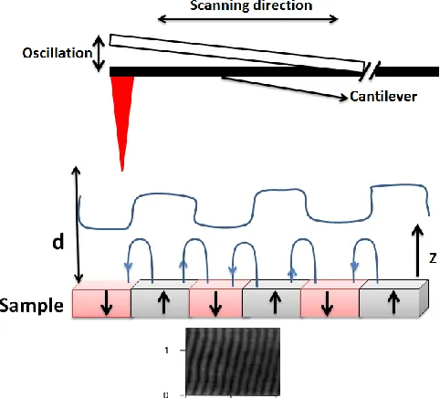
proportional to force gradient. In addition, the spring constant of the cantilever changed due to the Figure 2. 7: outline of MFM components and profile of force gradient from
38
interaction of the tip and sample. For example if k is a natural spring constant of cantilever, the modified
spring constant due to force gradient can be expressed as,
𝑘𝑓 = 𝑘 −
𝜕𝐹 𝜕𝑧
For the attractive interaction,𝜕𝐹𝜕𝑧> 0 and results cantilever spring softer. Similarly 𝜕𝐹𝜕𝑧< 0 represents the
repulsive interaction. Depending on whether attractive or repulsive interaction, different contrast are
observed which provides the information about the orientation of magnetization within sample. It will
be worth to mention that depending on the distance between and sample and probe tip, different type
of force contributes on force derivative. For example, if the gap between sample and tip is very close, it
probes van der-waals force. However, the magnetic force is long range in nature thus sample is probed
far away from sample surface (typically 100 nm). In figure2.7, systematic of the tip sample configuration
is depicted.
Let us consider slab which has magnetic domains are oriented out of plane. Depending on the
orientation of stray field, the deflection or attraction of the cantilever takes place. Then since we set the
set point fix, the path of the cantilever is traced which basically provides the information about the type
of stray field coming out from the sample. If the orientation of magnetization of tip and sample is same,
there will be black contrast and for opposite it will be white. The black and white stripe domain on
permalloy thin film is represented in the bottom of figure 2.7.
Mathematically, when the magnetic tip is brought close to the sample, the magnetic potential energy
can be expressed as [67]
39
Where M tip is the magnetization of tip of the probe and H sample is the stray field from the sample. Force
experience by the probe can be expressed as,
F = −∇E = −μ0∫ ∇(𝐌tip . 𝐇sample )dVtip
The integration is carryout throughout the tip of probe.
2.4 Dynamic characterization techniques
2.4.1 Ferromagnetic resonance
Resonance absorption of electromagnetic radiation within the ferromagnetic materials is called
ferromagnetic resonance [68]. In 1913, the first resonance spectrum was observed by Arkad’yev. The
important aspect of ferromagnetic resonance technique is that low amplitude of the excitation field
allows investigating the ground state properties of ferromagnetic materials without perturbation (more
details on chapter 1). For example, magnetization, magnetic anisotropies, g-factor and damping
constant can be determined with high precision. In addition FMR technique helps to develop microwave
devices such as circulator, microwave filter, oscillator, amplifier and spintronic devices. The systematic
40
2.8. The ground- signal- ground (GSG) type coplanar waveguide was connected with non-magnetic end
launch connectors followed by the coaxial cable and finally with the VNA ports. The samples were
fabricated with the help of e-beam lithography, sputtering and lift-off method on the top of the signal
line of CPW and process in details has been discussed in details in chapter 1.
The microwave frequency was swept at different frequency range depending on the nature of the
samples. The microwave current generates uniform ac magnetic field at the signal line of CPW. External
magnetic field was swept from positive saturation to negative saturation at field step of 5 Oe and the
orientation of the ac field and DC field was kept perpendicular to meet the requirement for FMR. The
scattering parameter (S21) was recorded as a function of microwave frequency and external field. The
41
Chapter 3: Exchange bias in (FeNi/IrMn)n multilayer films evaluated by static and dynamic
technique.
3.1Introduction to exchange bias effect
In this chapter, we will discuss the exchange bias in multilayer systems. Exchange bias is an interfacial
effect which exists at the interface between ferromagnetic [F] and antiferromagnetic [AF] specimen
[69]. In antiferromagnetic system, spins in one crystal plane are parallel however orientation of spins on
the adjacent plane antiparallel. For example, in case of MnO, spin on plane [111] are parallel but the
adjacent plane [111] has antiparallel spins [70]. On the other hand, ferromagnetic materials have
spontaneous magnetic moments. Therefore, when F and AF system are brought into contact and the
system is heated in presence of a magnetic field, it generates a unique effect at the interface, which
helps to pin the spins of ferromagnetic material at interface. This is called exchange bias. The first
signature of the coupling is the asymmetry of MHL with respect to origin [69]. The spin configuration of
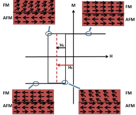
FM and AF at different external magnetic fields is represented in figure 3.1.
42
In figure 3.1, four different points on MHL loop are considered to explain how the spins orient at
different external magnetic field. Let us consider a state where the sample is positively saturated (the
spin configuration is presented on top right). The spins on FM materials are perfectly align along the
applied field direction. When magnetic field value decrease (top left), the spins on FM layer are ready to
flip to the opposite direction. However the switching fields are not symmetric with respect to origin. The
coupling strength between FM and AF determines the shift of the center of MHL loop from the origin. It
is called bias field, or, more specifically, exchange bias field. In figure 3.1 the exchange bias field is
denoted by HE. The similar process is represented on the right and left panel on the lower panel in figure
3.1 when the magnetic field is swept from negative to positive. The point to be noted here is that the
magnetization on AF is hard and external magnetic field cannot flip it. The AF layer is used only to pin
the FM layer.
Exchange bias effect has tremendous impact on technological applications. One of them is that this
effect can be used as sensor to read and write data in magnetic memory. In the following, we will be
discussing about a particular practical application in detail about uses of exchange bias effect as sensor
in Giant Magnetoresistance (GMR)[71]. In GMR head, there will be four thin layers. The first one is the
AFM layer and it is used to pin the spin of FM layer in specific orientation. Two F layers are separated by
43
non-magnetic thin layer and the schematic is presented in figure 3.2. The way GMR heads are used to
read and write in the magnetic medium is following. Generally the data are stored in the magnetic
domains of magnetic media. Magnetic stray field presents at the interface of magnetic domains and the
orientation of magnetic moments are represented with the arrows in figure 3.2. Depending on the
orientation of neighboring spins, the force between media and free layer would be attractive or
repulsive. As presented in figure 3.2, when stray fields switch the orientation of free FM layer, the
orientation of the spins of the pined and free layer will be parallel and the resistance across the
multilayer will be small. In contrast, when the orientation of spins on pined layer and free layer are
opposite, there will be maximum resistance. The change in resistance is measured electronically and the
maximum and minimum resistance can be read as 0 and 1 in data storage applications.
In addition, exchange-coupled multilayer systems are also ideal candidates for spin valve sensors,
microwave devices as well as in spintronic applications [72-77]. To enhance the applications of these
coupled systems, understanding the coupling mechanism and consequent effect on static and dynamic
properties is crucial. Extensive research in this regard has been done both theoretically as well as
experimentally [78-81]. For example, in previous studies, thickness of both F and AF layer was varied to
better understand thickness dependent exchange bias [82]. Temperature dependent studies on this
configuration have also been considered [78]. Misalignment of anisotropies, such as uniaxial and
unidirectional, because of the different thickness of the AF layer has been studied [82]. However, spin
frustration, nature of the magnetic domain, domain boundaries, and imperfection coupling between
F/AF layers significantly alter coupling scheme and it is hard to achieve theoretical expected exchange
bias results. In addition, experimental techniques, which are used to probe exchange bias, are also
44
In this study, we consider set of multilayer sample of F/AF thin layer. FeNi and IrMn were considered as
FM layer and AFM layer respectively. Comprehensive study of both static and dynamic properties has
been performed.
3.2 Sample preparation and characterization techniques:
A silicon substrate was coated with thermally oxidized 50nm thick SiO2. Multilayer films of composition
[FeNi(t nm)/IrMn(20 nm)]×n(t) where FeNi represent Ni(80%) and Fe(20%) were deposited on the
substrate using dc-triode sputtering method with base pressure of 3.0×10⁻⁹ Torr and Ar pressure at the
time of deposition was of 1.0×10⁻³ Torr. The deposition process was performed at room temperature. A
10 nm thick Ti layer was used as both a seed and capping layer. During the deposition process, the
external magnetic of field 250 Oe was applied along the long axis of slab to induce a longitudinal
magnetic anisotropy. The structural information for a set of three samples is presented in tabular form
below.
Sample FeNi
t( nm)
IrMn
t(nm)
Repetition number, n Full thickness (nm)
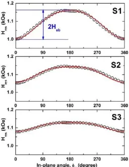
S1 20 20 10 400
S2 60 20 5 400
S3 80 20 4 400
The thickness of IrMn layers were kept constant for all samples. In-plane anisotropy and unidirectional
exchange bias were induced due to specific fabrication process.
The MHL and FORC measurements were implemented to carry out the static measurements. A
Princeton AGM-VSM magnetometer was used for room temperature studies. The external magnetic
![Figure 1.1: [a] Unit cell of Cobalt with easy and hard axis.[b] M vs H for two different axis of crystal](https://thumb-us.123doks.com/thumbv2/123dok_us/8922011.1842445/16.612.157.492.211.442/figure-unit-cell-cobalt-easy-hard-different-crystal.webp)
![Figure 1.11: [a] FVMSW [b] BVMSW [C] MSSW modes on thin film](https://thumb-us.123doks.com/thumbv2/123dok_us/8922011.1842445/33.612.151.372.141.452/figure-fvmsw-b-bvmsw-c-mssw-modes-film.webp)