Can the Threshold Performance of Maximum
Likelihood DOA Estimation be Improved by
Tools from Random Matrix Theory?
Yuri I. Abramovich
1,
Ben A. Johnson
2,∗1Institute for Telecommunications Research
University of South Australia, Mawson Lakes, SA 5045 Australia
2Colorado School of Mines, Golden, CO 80401 ∗Corresponding Author: [email protected]
Copyright c⃝2014 Horizon Research Publishing All rights reserved.
Abstract
For direction of arrival (DOA) estimation in the threshold region, it has been shown that use of Random Matrix Theory (RMT) eigensubspace estimates provides significant improvement in MUSIC performance. Here we investigate whether these RMT methods can also improve the threshold performance of unconditional (stochastic) maximum likelihood DOA estimation (MLE).Keywords
Signal Detection and Estimation, Maximum-likelihood Estimation, Random Matrix Theory1
Introduction
The “pre-asymptotic” performance of traditional stochastic (unconditional) MLE of DOAs formclosely-spaced Gaussian signals immersed in white Gaussian noise using an M-sensor array and a finite number T independent identically distributed (i.i.d.) training samples continues to be the subject of investigations [3–5, 15] despite being a relatively “old” problem [16]. The main reason, as formulated in [4], is that in the pre-asymptotic domain, “no general non-asymptotic results are[currently]available for the performance evaluation of the ML method, and each problem requires a special investigation”.
As an alternative, instead of focusing on the accurate non-asymptotic analysis, one may consider the asymptotic model where both quantitiesM andT grow without bound, while their quotient converges to a fixed finite quantity:
M, T → ∞, M
T →c, 0< c <∞ (1)
This condition is known as the Kolmogorov asymptotic condition [6], and underpins a field of analysis referred to as Generalized Statistical Analysis (GSA) or Random Matrix Theory (RMT). Of course, in any practical situation, one deals with finiteM andT values, and therefore generalized “G-asymptotic” (i.e. asymptotic per the conditions in (1)) results may still not be sufficiently accurate. However, in numerous studies, it has been demonstrated that estimators that are consistent G-asymptotically are more robust in the presence of finite samples T than other estimators which are only consistent forT → ∞,M =constant [6, 10, 11, 18].
Specifically, let us suppose that i.i.d. observationsx1, . . . ,xT of random vectorξwith dimensionM are given,
and we wish to estimate some valueφ(RM), whereφis a continuous function of the entries of the (true) covariance
matrixRM of vectorξ. IfT is large andM is fixed and does not change asT grows (i.e. the standard asymptotic
case), then as an estimator ofφ(RM), we may takeφ( ˆRM), where
plim
T→∞
φ( ˆRM) =φ(RM) (2)
and ˆRM is the standard sample covariance matrix for zero-mean data (= T1 ∑Tj=1xxH). Moreover, if xj, j =
1, . . . , T is a set of i.i.d. complex (circular) Gaussian samples (i.e. xj ∼ CN(0, RM)), then ˆRM and φ( ˆRM) are
not only consistent (in the standard asymptotic framework), but also the maximum likelihood estimate ofRM and
(1). There, for a wide range of functionsφ(RM), one can find a measurable functionψof the entries of the matrix
RM for which
plim
M,T→∞
[φ( ˆRM)−ψ(RM)] = 0. (3)
But in general, the functions φ(RM) and ψ(RM) do not coincide, in which case φ( ˆRM) is not necessarily a G-consistent estimate of φ(RM). However, with the help of function ψ(RM), one may try to find a measurable functiong( ˆRM) such that
plim
M,T→∞
[g( ˆRM)−φ(RM)] = 0. (4)
and where the distribution of normalized differenceg( ˆRM)−φ(RM) is asymptotically normal. The functiong( ˆRM) is then called a G-estimator [6], and is consistent under condition (1).
In [10,11], this RMT methodology has been used to find G-estimates of eigenvalues for a covariance matrix with known multiplicity of its eigenvalues. Specifically, for anM-variate covariance matrixRM, letγ1< γ2< . . . < γM
be the set ofM distinct eigenvalues (1≤M ≤M) after accounting for individual multiplicityKm of theM true eigenvalues (i.e. ∑Mm=1Km=M). Associated with each eigenvalue γm, there is a complex subspace of dimension Km. This subspace is determined by anM×Kmmatrix of corresponding eigenvectors, denoted byEm, such that
EH
mEm =IKm. Note that this specification is unique up to right multiplication by the orthogonal matrix, and
therefore the problem of eigendecomposition for the matrixRM
RM =
M
∑
j=1
γjEjEjH (5)
is more convenient to formulate as a problem of estimation of orthogonal projection matrices, defined as
Pm=EmEmH, m= 1, . . . , M , (6)
given the sample covariance matrix ˆRthat has the eigendecomposition ˆ
R=
M
∑
j=1
ˆ
λjUˆjUˆjH (7)
To use this eigendecomposition to estimate the orthogonal projection matricesPm, letKm be a set of indices
Km=
m∑−1
j=1
Kj, m∑−1
j=1
Kj+ 1, . . . , m
∑
j=1
Kj
(8)
with the cardinality ofKmequal to the multiplicity of the eigenvalueγm, namelyKm.
The classical (and indeed maximum likelihood for multivariate Gaussian observations) estimator of the m-th eigenvalue and orthogonal projection matricesPmin (6) is given by
ˆ
γmM L= 1
Km
∑
k∈Km
ˆ
λk; ˆPmM L=
∑
k∈Km
ˆ
UkUˆkH (9)
One can see that ˆγM L
m and ˆPmM L are specified as φ( ˆRm) in (2) and indeed are strongly T-consistent (and ML)
estimates ofγmandPm.
Yet in Theorem 2 of [10], X. Mestre proved that under certain conditions (As1-As4), the traditional estimators of eigenvalues and eigensubspaces (ˆγM L
m and ˆηjM L=S1H
∑
k∈Km
ˆ
UkUˆkHS2, respectively, where S1 and S2 are two
M×1 deterministic vectors) can be shown to converge under condition (1) (i.e. M, T → ∞withM/T =cconstant and finite) to:
|γˆmM L−γM Lm | →0 and|ηˆjM L−ηM Lm | →0 (10) where the (non-random) valuesγM Lm andηM Lm are defined as
γM Lm =γm
1− c
M M
∑
r=1
r̸=m Kr
γr γr−γm
(11)
and
ηM Lm =
M
∑
k=1
wm(k)SH1 EkEkHS2 (12)
wm(k) =
{
1−K1
m
∑M r=1
r̸=mKr
(
γm γr−γm −
µm γr−µm
)
k=m
γm γr−γm −
µm
γr−µm k̸=m
whereµmis them-th solution to the following equation inµ:
1
M M
∑
r=1
Kr γr
γr−µ =
1
c (14)
under the convention µ1 < µ2 < . . . < µM. Thus, the traditional ML estimators for ˆγmM L and ˆηM Lm are not
G-consistent estimates, and therefore could potentially be improved within the RMT methodology1. “Improved”
G-consistent estimates for γm andPmunder the conditions (As1-As4) have been derived by X. Mestre, Theorem 3 in [10]:
ˆ
γmG = T
Km
∑
k∈Km
(ˆλk−µkˆ ),
ˆ
ηmG =
M
∑
k=1
ρm(k)S1HUkˆ UˆkHS2;
(15)
where
ρj(k) =
{
−φm(k), k /∈ Km
1 +ψm(k), k∈ Km φm(k) = ∑
r∈Km
(
ˆ
λr
ˆ
λk−λˆr
−ˆ µrˆ
λk−µˆr
)
ψm(k) = ∑
r /∈Km
(
ˆ
λr
ˆ
λk−λˆr
− ˆ µrˆ
λk−µˆr
)
(16)
and ˆµ1≤µˆ2≤ · · · ≤µˆM are the real-valued solutions to the following equation in ˆµ:
1
M M
∑
k=1
ˆ
λk
ˆ
λk−µˆ
=1
c; c= M
T (17)
One can prove (see [10]) that for any fixedM, as T → ∞, we have ˆ
µk →λk, Tˆ (ˆλk−µkˆ )→λkˆ (18)
and therefore
ˆ
γmG →
1
Km
∑
k∈Km
ˆ
λk= ˆγmM L (19)
On the other hand,φm(k)→0 andϕm(k)→0, which implies that ˆηmG →ηˆmM L, as T → ∞.
Therefore, the RMT methodology provides a unique set of G-consistent estimates for ˆγG
m and ˆηmG that tend to
the classical MLE estimates under traditional asymptotic assumptions (M = constant, T → ∞). Specifically, the G-consistent MUSIC (or G-MUSIC) pseudo-spectrum estimate
ˆ
η1G(θ) =
M
∑
k=1
ρ1(k)SH(θ) ˆUkUˆkHS(θ) (20)
has been suggested in [9] and demonstrated significant performance improvement compared with the traditional MUSIC function ˆη1M L(θ).
Recently in [8], we showed that for closely spaced sources, despite the substantial improvements demonstrated by G-MUSIC (20) with respect to conventional MUSIC, the “threshold” performance of G-MUSIC (where the estimator’s mean squared error departs rapidly from the Cram´er-Rao lower bound as SNR and/or sample support is reduced) remains significantly worse than performance of the rigorously implemented (via global search) ML DOA estimation. Since the RMT-methodology, and specifically the G-consistent estimates in (15), are able to improve conventional MUSIC performance and differ from the traditional ML eigenvalue and subspace estimates, it is quite legitimate to investigate whether these estimates may be used to improve the threshold performance of ML DOA estimation itself. In this correspondence, we try to address this question.
1Note that forS
1 =S2 =S(θ) whereS(θ) is anM-element antenna steering (manifold) vector specified by the DOAθ, and for
2
G-asymptotic ML DOA Estimation (G-MLE) Formulation
For the stochastic (unconditional) ML model under consideration, the set of T i.i.d. data xj ∈ CN(0, R0),
j= 1, . . . , T is described by the true/exact covariance matrixR0, comprised of mindependent planewave sources
with direction of arrivalθm, embedded in white noise. Under this model, the traditional ML DOA estimates are found as the global maximum of the stochastic (unconditional) likelihood function (LF) computed for the model covariance matrixR(Ωm), uniquely specified by 2m+ 1 parameters in Ωm(msource DOAs and powers as well as
the noise power) and denotedL[R(Ωm)]:
ˆ
Ωm= arg max
Ωm
L[R(Ωm)],
L[R(Ωm)] =
[
exp[−trR−1(Ω
m) ˆR] πMdetR(Ω
m)
]T (21)
or, equivalently, as the minimum of the (scaled)2 log-likelihood function (LLF)
lL[R(Ωm)] =
trR−1(Ω
m) ˆR
M +
log detR(Ωm)
M (22)
Note that for any givenR(Ωm), the LLF (22) may be viewed as the ML estimate of the function φ[R(Ωm), R0]≡φ[R−
1
2(Ωm)R0R− 1
2(Ωm)] =
= 1
M tr [R
−1
2(Ωm)R0R− 1
2(Ωm)] + 1
M log detR(Ωm) (23)
with an unknownR0, here represented by its generic (positive definite Hermitian, forT ≥M) ML estimate sample
covariance matrix ˆRformed from the training dataxj.
Since the likelihood function (22) is just φ( ˆRM(Ωm)) (per the notation in (2)), under the RMT methodology,
we need to construct the G-consistent estimateg( ˆRM(Ωm)) (per the notation in (4)) of the functionφ0(the portion
ofφfrom (23) dependent onR0, which can be simplified to M1 trR−1(Ωm)R0).
Yet, according to Lemma 3.1 in [6] (see eqn. 3.10, p. 182), for a very broad class of empirical covariance matrices that embraces the complex Wishart case
ˆ
RM(Ωm) =
1
TR
−1
2(Ωm)R 1 2
0CRˆ
1 2
0R−
1
2(Ωm); ˆC∼ CW(M, T, IM), (24)
under the Kolmogorov asymptotic condition (1), the following property is proven: plim
T→∞,M T→c
[
1
M tr ˆRM −
1
ME( tr ˆRM)
]
= 0, (25)
whereE(·) is the expectation operator and CW(M, T, IM) is the complex Wishart distribution [7].
This property means that for the functionφ0, we have aspecial casewhere its G-consistent estimateg( ˆRM(Ωm))
coincides with its ML estimateφ0( ˆR):
g( ˆRM(Ωm)) =φ( ˆRM(Ωm)) =
1
M tr [R
−1(Ω
m) ˆR] (26)
In essence, the property (25) means that for the multivariate complex Gaussian data case, the (scaled) uncon-ditional log-likelihood function (22) may be treated as the ML estimate and at the same time, the G-consistent estimate of the functionφ[R(Ωm), R0] given in (23).
Lemma 3.1 from [6], and more importantly, its interpretation as G-consistency of the standard log-likelihood function3, leaves an apparent contradiction which needs to be resolved. Specifically, since according to Theorem 2
from [10], individual ML estimates of eigenvalues are not G-consistent and can be improved, per (15). At the same time, thesum of all eigenvalues (i.e. the sample covariance matrix trace) is G-consistent, and therefore cannot be improved within the RMT methodology4. This contradiction could be resolved by the direct proof that the sum
2This scaling by the factor 1/Mis immaterial for a fixedM, but is subsequently required for G-asymptotic analysis with (M, T)→ ∞,
M/T→c, forlL[R(Ωm)] to remain finite asM→ ∞
3It is important to emphasize that G-consistency of the likelihood function (or the G-MUSIC function, for that matter) does not
imply that the resultant DOA estimates are always G-consistent as well. On the contrary, the fact that the globally optimal ML DOA estimates (as well as the G-MUSIC DOA estimates) exhibit performance breakdown in their respective threshold regions demonstrates that G-consistency of the likelihood or G-MUSIC function is only a necessary, but not at all sufficient condition for G-consistent DOA estimation.
4While Theorem 3 in [10], provides a unique set of G-consistent estimates (15) within the RMT methodology, it does not resolve
of G-consistent individual eigenvalue estimates ˆγG
min (15) is strictly equal to the sum of sample eigenvalues ˆλk of
ˆ
RM(Ωm), ie.
M
∑
m=1
KmˆγmG = M
∑
k=1
ˆ
λk= tr [ ˆRM(Ωm)] (27)
According to (15), we therefore have to prove that
Theorem 1 Under conditions As1-As3 in [10], the estimate
M
∑
m=1
KmˆγmG =T( M
∑
k=1
ˆ
λk− M
∑
k=1
ˆ
µk) = M
∑
k=1
ˆ
λk (28)
is the G-consistent estimate of the trace ofRM, regardless of the “eigenvalue splitting condition” As4.
The proof of this equivalence is shown in Appendix A, and shows that the trace of a sample matrix ˆRis always the G-consistent estimate of the trace of the original (true) covariance matrixRM, even when for some individual eigenvalues of this matrix, their G-consistent estimates may not exist due to As4 not being satisfied.
As an aside for the interested reader, Mestre’s assumptions As1 to As3 (the details of which are provided in [10]) impose general conditions on the covariance matrix and eigenvalues which are always meet under our problem with the sample Wishart matrix ˆRM(Ωm), but assumption As4 may or may not be met. The physical
meaning of the As4 condition, also referred to as the eigenvalue splitting condition, is that the asymptotic eigenvalue distribution of ˆR can be considered as a collection of clusters, each one centered around a different eigenvalue of
RM =ERˆM =R− 1
2(Ωm)R0R− 1
2(Ωm). The size of the support of these clusters depends on the ratio of the number
of sensors/antennas to the number of samples (ie. the ratioc=M/T) from which ˆR is constructed. If the ratio
M/T is high, the clusters with close eigenvaluesγj ofRM may merge and be represented by a single estimate with a certain “multiplicity”K. If, on the contrary, the ratioM/T is low, each sample eigenvalue ˆλk will be associated
with a different distinct cluster, well separated from the rest of the sample eigenvalue distribution.
This analysis provides an answer, therefore, to the main question posed in the title of this correspondence: Within the existing RMT framework, “improved” G-consistent estimates of individual eigenvalues ˆγG
mand bilinear
forms ˆηG
m given in (15) cannot make the traditional log-likelihood function “more G-consistent”, and therefore
provide any improvement into the threshold performance of ML DOA estimation, in full correspondence with Lemma 3.1 from [6] shown in (25) above.
To confirm this further and support numerical evaluation, we still may consider an alternative reconstruction of the G-consistent log-likelihood function using the individual estimates (15) in a manner similar to the G-MUSIC derivation in [9]. Assuming that the “eigenvalue splitting condition” As4 from [10] is satisfied for all the (m+ 1) different eigenvalues5, we may construct the G-LLF (log likelihood function) as
g0[R(Ωm)] =
1
M trR
−1(Ω
m) ˆRGm, Rˆ G m=
m∑+1
j=1
ˆ
λGjPˆjG. (29)
where, based on (15), G-consistent estimates of the eigenspacePj inR0(R0=λ1P1+
∑m+1
j=2 λjPj) are given by
ˆ
PjG=
M
∑
k=1
ρj(k) ˆUkUˆkH; ˆR= M
∑
j=1
ˆ
λjUˆjUˆjH (30)
Recall that G-MUSIC was calculated as per (20), and therefore (29)-(30) resemble this construction, but with some differences. First of all, in contrast to standard eigendecomposition, we note that individual eigen-subspace estimates ˆPG
j in (30) are no longer mutually orthogonal, though they can be shown to sum to the
identity matrix since the weights ρj(k) in (16) sum to unity. Therefore, if we introduce the diagonal matrix D(j)≡diag[ρj(1), . . . , ρj(M)], we immediately discover that according to (30), we get
ˆ
RGm= ˆU
m∑+1
j=1
ˆ
λGjDj
UˆH. (31)
While individual (G-consistent) estimates ˆPG
j in (30) are different from the ML estimates ˆPj=
∑
k∈Kj
ˆ
UkUˆH k , the
eigenvectors in ˆRG
mare exactly the same as in the ML estimation ˆRM Lm (Theorem 9.3.1 in [13]). 5Recall thatR
0 (as opposed to the whitened covariance matrix RM) consists of an m dimensional signal subspace and a noise
Let us demonstrate that “reconstructed” eigenvaluesλR k in
∑m+1
j=1 λˆ
G
jDj= diag[ˆλR1, . . . ,λˆRk] (at least G-asymptotically)
tend to the same limit as the (not G-consistent) MLE estimate ˆγkM L:
lim
M,T→∞ M/T→c
ˆ
λRk ⇒ lim
M,T→∞ M/T→c
ˆ
γjM L=γk
1 + c
M m∑+1
r=1
r̸=k
Kr γr
γr−γk
(32)
Using (15)-(16), for the noise subspace eigenvalues (ˆλR
1, . . . ,λˆRM−m), we get
ˆ
λRk = ˆλGk
1 +
M
∑
r=1
r̸=k
ˆ
λr
ˆ
λk−ˆλr
− ˆ µrˆ
λk−µˆr
−
−
M
∑
r=1
r̸=k
ˆ
λGr
[
ˆ
λr
ˆ
λk−λˆr
−ˆ µrˆ
λk−µˆr
]
, (33)
fork= 1, . . . ,(M−m) and with ˆλG
1 = ˆλG2 =. . .= ˆλGM−m, which is identical to
ˆ
λRk = ˆλGk + ˆλk M
∑
r=1
r̸=k
(ˆλG k −λˆ
G
r)(ˆλr−µˆr)
(ˆλk−λrˆ )(ˆλk−µrˆ ), k= 1, . . . ,(M −m). (34)
According to (15), for signal subspace eigenvalues (r≥M−m), we get ˆλr−µˆr= T1ˆλGr, and therefore we have
ˆ
λRk = ˆλGk −
ˆ
λk T
M
∑
r=1
r̸=k
(ˆλGk −ˆλGr)ˆλGr
(ˆλk−ˆλr)(ˆλk−µrˆ ). (35)
Note that for ˆλr−1 ≪µrˆ <ˆλr and ˆµr → TT−1λrˆ when As4 is strongly met. Therefore the difference between
(35) and the expression (see (11) and (32))
ˆ
λRk = ˆλGk −
ˆ
λG k T
m∑+1
r=1
r̸=k
(ˆλG k −λˆ
G r)ˆλGr
(ˆλG
k −ˆλGr)(ˆλGk −λˆGr)
(36)
that strictly tends toγM Lk in (11) under asymptotic condition (1), is only a difference of the second order (in T1) magnitude.
Therefore, the reconstructed noise subspace eigenvalues in ˆRG
M (31) G-asymptomatically are not strictly
iden-tical, but the fluctuations around its asymptotic value γM L1 is quite negligible. For signal subspace eigenvalues, these fluctuations are even less significant, which may be demonstrated by derivations similar to those above.
While it would be more satisfying if ˆλRk was found to be strictly equal to the ML version ˆγkM L, this is not the case, as observed by other researchers in the field [12]. But practically speaking, it is not significant that non G-consistent estimates ˆγM L
k are replaced in (29) by (slightly) different non G-consistent estimates ˆλRk. The main
point is that the reconstruction in (29) using the G-consistent estimates of eigenvalues and eigenvectors (15) should be at best as efficient as the conventional accurate MLE DOA estimate.
Therefore, the conducted analysis has demonstrated how and why the G-consistent individual estimates of eigenvalues and eigenvectors help to improve MUSIC threshold performance, but still lead to the traditional ML performance. This property is proven rigorously for direct G-consistent estimation of M1 tr (R−1(Ω
m)R0), and in
first order (in T1) approximation for the reconstruction approach in (29). Let us now support these theoretical findings by empirical results.
3
Numerical Evaluation
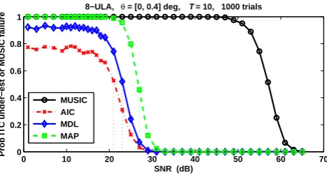
Here, we seek by simulation to demonstrate, using direct exhaustive search for the global maximum of the likelihood function and its reconstructed G-modification, that their DOA estimation performance in the threshold region is identical. For this analysis, we have selected the same scenario as in [1] withM = 8 sensor ULA,T = 10 i.i.d. training samples and two equipower sources (p1 = p2) with DOAs {0o,0.4o} in white noise powerp0 = 1.
The number of sourcesm= 2 is limited by the computational load associated with the exhaustivem-dimensional search for the LF global maximum, but still demonstrates the relevant MLE threshold behavior. For this scenario, the CRB resolution limit (as predicted by the CRB RMSE of 0.2o, derived in more detail in [1]) occurs at an SNR
0 10 20 30 40 50 60 70 0
0.2 0.4 0.6 0.8 1
SNR (dB)
Prob ITC under−est or MUSIC failure
8−ULA, θ = [0, 0.4] deg, T = 10, 1000 trials
[image:7.595.174.408.55.180.2]MUSIC AIC MDL MAP
Figure 1. Sample MUSIC breakdown for closely spaced sources. Note the SNR gap between reliable detection using ITC and reliable
estimation using MUSIC.
Fig. 1 plots the probability of underestimating the correct number of sources as a function of SNR for the AIC, MDL, and MAP information theoretic criteria (ITC). The same figure shows the sample probability of conventional MUSIC breakdown, which illustrates the well-documented fact that MUSIC “breaks” at SNR values significantly larger than the actual MLE threshold [8]. In this paper, we examine the performance at εITC = 30dB, where
Fig. 1 shows the reliable detection of the correct number of sources m= 2, but the ML DOA estimate itself is questionable.
It can be separately confirmed, following the methodology in [10], that for this scenario, the eigenvalue splitting condition As4, required for G-consistency of the eigenvalue estimation, are met for the 30dB case in this scenario. The fact that this condition is met here comes with no surprise. Indeed, the reliable detection of the correct number of sources m= 2 at this SNR already implies that the cluster of noise subspace sample eigenvalues (ˆλ1 to ˆλ6) is
reliably separated from the cluster of the smallest signal eigenvalue ˆλ7. Sinceλ8≫λ7for our scenario with closely
spaced sources, it is really the separation between theλ7 cluster and the noise subspace one (λ1=· · ·=λ6= 1),
which is of concern for evaluation of the As4 condition.
0.1 1 10 100 1000 10000 0
0.05 0.1 0.15 0.2 0.25
sample pdf
Eigenvalue
8−ULA, θ = [0, 0.40] deg, T = 10, 30dB SNR, G, 500−0 {U#30}
[image:7.595.178.404.400.520.2]G−asym Eig Standard Eig
Figure 2. Sample p.d.f.s for the eigenvalues of ˆRG
m
We therefore examine the eigendecomposition of the G-reconstructed covariance matrix ˆRG. As predicted, the
eigenvectors of ˆRm and ˆRGm are exactly the same, and only the eigenvalues differ slightly (and then only in the
noise subspace). The two subspace eigenvalues are also well separated both from each other and the noise subspace eigenvalues. While in ˆRmthe noise subspace is described by a single value (= M1−m
∑M−m
j=1 λˆj), in ˆRGmthey remain
close but not precisely equal to ˆλ1 (i.e. eig1( ˆRGm)<ˆλG1 <eig6( ˆRGm)). This is demonstrated in Fig. 2, where we
introduce sample p.d.f.s for eig7( ˆRGm), eig8( ˆRGm), and the noise eigenvalues eign( ˆRGm) = (eig1( ˆRGm),. . . , eig6( ˆRGm)),
where here we treat as the noise subspace eigenvalue in ˆRG
many one of its six smallest eigenvalues. The p.d.f.s for
ˆ
λ1 and eign( ˆRGm) practically coincide.
While Fig. 2 does demonstrate minor variations in the noise subspace eigenvalues in ˆRG
m around the single
noise subspace eigenvalue ˆλG
1 in ˆRm, caused by finiteT andM values, these variations are very unlikely to result
in any noticeable changes in DOA estimation performance when ˆRG
mis used instead of ˆRm or ˆR in the likelihood
function, simply because even larger variations of noise subspace eigenvalues in ˆR around a single ML estimate (= M1−m∑jM=1−mλˆj) in ˆRmare also not associated with any DOA ML estimation performance degradation.
Yet, since all the conditions (As1-As4) of the Theorem 3 [10] are met, we can expect that these minor variations do result in improved individual eigenvalue ˆλGj and eigensubspace ˆPjG estimation accuracy. To confirm this, we repeat the analysis conducted in [10], where to assess the quality of the eigensubspace estimates, Mestre introduced anorthogonality factor:
O(j) = |tr [Pj ˆ
Pj]|
|tr [In−Pj] ˆPj|. (37)
(either standard ML ones or the G-consistent ˆPG
j ones). This orthogonality factor is the ratio of the total power of
the estimated subspace ˆPjthat resides in the true subspacePjto the power of its “leakage” into the true orthogonal subspace [IM −Pj].
5 10 15 20 25 30 35 40 45
0 0.05 0.1 0.15 0.2
sample pdf
orthogonality
2
8−ULA, θ = [0, 0.40] deg, T = 10, 30dB SNR, G, 500−1 {U#30}
Rhat Ghat
10 15 20 25 30 35 40 45 50 55
0 0.05 0.1 0.15 0.2
sample pdf
orthogonality
3
8−ULA, θ = [0, 0.40] deg, T = 10, 30dB SNR, G, 500−1 {U#30}
[image:8.595.61.552.110.232.2]Rhat Ghat
Figure 3. Sample p.d.f.s for MLE and GMLE orthogonality factors for the two signal eigenvectors.
The estimate ˆPG
j (as defined in (30)) is “better” than the MLE ˆPj, defined as ˆP1=
∑6
j=1Ujˆ UˆjH; ˆP2= ˆU7Uˆ7H;
ˆ
P3 = ˆU8Uˆ8H if, with high probability, the respective orthogonality factor is greater. In Fig. 3, we introduce
sample p.d.f.s for the orthogonality factorO(j) andO(j)G, averaged over the same 500 Monte-Carlo trials for the
SNR=30dB case. Similarly to [10], we observe that the G-consistent subspace estimate achieves a much higher orthogonality factor than the traditional ML sample estimator, indicating a better capacity to estimate subspaces, and therefore better accuracy for subspace-based DOA estimation techniques such as MUSIC.
To demonstrate, we compare the results of exhaustive global maximum search for the conventional (normalized) likelihood function (ratio):
LR[R(Ωm)] =
detR−1(Ωm) ˆReM etrR−1(Ω
m) ˆR
(38)
and its G-asymptotic counterpartGLR[R(Ωm)] constructed using ˆRGminstead of ˆR.
−6 −4 −2 0 2 4 6
10−3 10−2 10−1 100
sample pdf
θ (deg)
8−ULA, θ = [0, 0.40] deg, T = 10, 30dB SNR, R, 500 {U#30}
−6 −4 −2 0 2 4 6
10−3 10−2 10−1 100
sample pdf
θ (deg)
8−ULA, θ = [0, 0.40] deg, T = 10, 30dB SNR, G, 500−1 {U#30}
Figure 4. Sample p.d.f.s for MLE and GMLE DOA estimation at 30dB SNR; a- ˆRm, b- ˆRGm.
This global optimization is performed in two steps. In step 1, we find the global extremum over a fine grid on a half-plane (θ1 < θ2), and in step 2, we conduct local optimization over the parameters θ1 < θ2 as well as
the two source powers using the MATLAB fmincom routine. The white noise power is assumed known a priori
and set to unity. More details on the optimization routine and MLE results can be found in [1, 2, 14]. Due to our convention that ˆθ1<θˆ2, the DOA sample distributions illustrated by Fig. 4 overlap, since for scenarios with
very closely spaced sources, over the 500 trials, the minimum ˆθ2 was sometimes less than the maximum ˆθ1, even
though on each individual trialθ1was less thanθ2. One can see that the distribution for the DOAs derived using
the standard LR (38) and the G-asymptotic counterpart are practically indistinguishable, as are any moments of these distributions. Moreover, in addition to the identical statistical performance of the DOA estimates, identical individual estimates were registered in a trial-by-trial basis.
In addition to the illustrated results, the same results were observed at several higher SNRs, and were also the same when the ML covariance matrix estimate ˆRm =∑Mk=1γˆmM LPmM L was used. Finally, in a completely ad-hoc
“mix and match” approach, we also assigned the G-consistent eigenvalue estimates ˆλG
1 (the G-consistent noise
power estimate), ˆλG
2 and ˆλG3 (15) to the maximum likelihood (mutually orthogonal) eigensubspaces ˆP1, ˆP2, and
ˆ
P3 and once again did not record any DOA estimation improvements, showing that the minor variations in noise
subspace eigenvalues in ˆRG
[image:8.595.63.550.440.580.2]4
Concluding Remarks
The theoretical results from RMT and their examination by direct Monte-Carlo simulations has confirmed that for Gaussian sources in Gaussian noise, ML DOA estimation in the so-called “threshold” region is not improved by use of recent results from Random Matrix Theory. More specifically, we demonstrated that the Girko Lemma 3.1 from [6] implies that for the multi-variate (complex) Gaussian data case, the stochastic (unconditional) likeli-hood function is both aT-consistent and G-consistent estimate of the function 1/Mtr [R−1(Ωm)R0], where R0 is
represented by a set ofT i.i.d. training vectorsxj.
We demonstrated that in full accordance with this Lemma, an alternative reconstruction of the log-likelihood function using individually G-consistent estimates of eigenvalues and eigenvectors does not improve DOA estimation threshold performance, despite the fact that these individual G-consistent estimates are more accurate than their corresponding ML estimates. Thus, the demonstrated in [9–11] improvement in MUSIC performance delivered by the G-consistent estimates of the individual noise eigensubspace is not at odds with the lack of improvement in MLE performance.
While applicable to arbitrary parametric description of the covariance matrix R0, these results should not
be extended beyond the multivariate (complex) i.i.d. Gaussian case without detailed examination. Finally, it is important to stress that our results are confined to the currently (in [10]) unique set of G-consistent eigenvalue and eigenvector estimates, and therefore the broader question on whether the threshold performance of ML DOA estimation can be improved by some other technique remains open.
Acknowledgements
The authors express their gratitude to Dr. Xavier Mestre of the Telecommunications Technological Center of Catalonia (CTTC) for his guidance on RMT results.
Appendix
Proof of Theorem 1
The G-consistent eigenvalue estimators defined in Theorem 3 in [10] ((15) in the main body of the paper) can be restructured as
M
∑
m=1
KmˆγmG =T( M
∑
k
ˆ
λk− M
∑
k
ˆ
µk), (4.1)
and therefore we have to prove that
T M
∑
k=1
ˆ
µk= (T−1)
M
∑
k=1
ˆ
λk. (4.2)
Given eqn. (17) in the main body of the paper, we may define
T M
∑
k=1
ˆ
µk =
M
∑
k=1
M
∑
m=1
ˆ
λmµkˆ ˆ
λm−µˆk
. (4.3)
Substitution shows that instead of the form in eqn. (17), ˆµ1, . . . ,µˆM can be introduced as the roots of the following
polynomial:
Q(µ) =
M
∏
k=1
(ˆµk−µ)
=
M
∏
j=1
(ˆλk−µ)− 1
T M
∑
r=1
ˆ
λr M
∏
j=1
j̸=r
(ˆλj−µ)
(4.4)
where the right-hand side expression is obtained from eqn. (17). EvaluatingQ(µ) atµ=λm, we obtain
M
∏
k=1
(ˆλm−µkˆ ) = 1
T
ˆ
λm M
∏
j=1
j̸=m
On the other hand, observing the form of the derivative ofQ′(µ):
Q′(µ) =−
M ∑ l=1 M ∏ k=1
k̸=l
(ˆµk−µ) =
=− M ∑ l=1 M ∏ j=1
j̸=l
(ˆλj−µ) +
1 T M ∑ r=1 ˆ λr ∑ l=1
l̸=r M
∏
j=1
j̸=r j̸=l
(ˆλj−µ)
(4.6)
and evaluating it atµ= ˆλm, we obtain M ∑ l=1 M ∏ k=1
k̸=l
(ˆµk−ˆλm) =−
M
∏
j=1
j̸=m
(ˆλj−λmˆ )− 1
T
ˆ
λm∑
l=1
l̸=m M
∏
j=1
j̸=m j̸=l
(ˆλj−ˆλm)
− 1
T
∑
r=1
r̸=m
ˆ
λr M
∏
j=1
j̸=r j̸=m
(ˆλj−ˆλm) (4.7)
Dividing both sides of (4.7) by∏Mj=1
j̸=r,m
(ˆλj−ˆλm) and using (4.5) to simplify the left-hand side, we obtain
1 T M ∑ l=1 ˆ λm ˆ
λm−µˆl
= 1− 1
T
∑
r=1
r̸=m
ˆ
λm+ ˆλr
ˆ
λr−λˆm
(4.8)
(Note that (4.4)-(4.8) follow Appendix IV in in [10]). On the other hand, from (4.3) we get
M ∑ k=1 M ∑ j=1 ˆ
λkµjˆ ˆ
λk−µˆj
= M ∑ k=1 ˆ λk ∑M
j=1
ˆ
λk
ˆ
λk−µˆj
−1
(4.9)
From (4.8), it then follows that
M ∑ k=1 ˆ λk ˆ
λk−µjˆ =T−
M
∑
r=1
r̸=k
ˆ
λk+ ˆλr
ˆ
λr−λkˆ (4.10)
Since
M
∑
r=1
r̸=k
ˆ
λk+ ˆλr
ˆ
λr−ˆλk
+ 1−1 =
M
∑
r=1
r̸=k
(
2ˆλr
ˆ
λr−λˆk
−1 ) (4.11) we get M ∑ k=1 M ∑ j=1 ˆ
λkµjˆ ˆ
λk−µˆj
= (T−M+M −1)
M ∑ k=1 ˆ λk− M ∑ k=1 M ∑ r=1
r̸=k
2ˆλkλrˆ
ˆ
λr−ˆλk
. (4.12)
But for ˆλk >0, the following identity is true (see [10]) M ∑ k=1 M ∑ r=1
r̸=k
ˆ
λkˆλr
ˆ
λr−λkˆ = 0. (4.13)
Therefore, we get
T M
∑
k=1
ˆ
µk = (T−1)
M
∑
k=1
ˆ
λk (4.14)
REFERENCES
[1] Y.I. Abramovich, B.A. Johnson, and N.K. Spencer. Statistical nonidentifiability of close emitters: Maximum-likelihood estimation breakdown. InProc. EUSIPCO-2009, pages 1968–1972, Glasgow, UK, 2009.
[2] Y.I. Abramovich, B.A. Johnson, and N.K. Spencer. Statistical nonidentifiability of close emitters: Maximum-likelihood estimation breakdown and its GSA analysis. InProc. ICASSP-2009, pages 2133–2136, Taipei, Taiwan, 2009.
[3] F. Athley. Threshold region performance of maximum likelihood direction of arrival estimators. IEEE Trans. Signal Processing, 53(4):1359–1373, Apr 2005.
[4] P. Forster, P. Larzabal, and E. Boyer. Threshold performance analysis of maximum likelihood DOA estimation. IEEE Trans. Sig. Proc., 52(11):3183–3191, Nov 2004.
[5] A.B. Gershman. Pseudo-randomly generated estimator banks: a new tool for improving the threshold performance of direction finding. IEEE Trans. Sig. Proc., 46(5):1351–1364, May 1998.
[6] V.L. Girko. An Introduction to Statistical Analysis of Random Arrays. VSP, Utrecht, Netherlands, 1998.
[7] R.A. Janik and M.A. Nowak. Wishart and anti-Wishart random matrices. J. Phys. A, 36:3629–3637, 2003.
[8] B.A. Johnson, Y.I. Abramovich, and X. Mestre. MUSIC, G-MUSIC, and maximum-likelihood performance breakdown.
IEEE Trans. Sig. Proc., 56(8):3944–3958, August 2008.
[9] X. Mestre. An improved subspace based algorithm for small sample size regime. InProc. ICASSP-06, Toulouse, 2006.
[10] X. Mestre. Improved estimation of eigenvalues and eigenvectors of covariance matrices using their sample estimates.
IEEE Trans. Info. Theory, 54(11):5113–5129, November 2008.
[11] X. Mestre. On the asymptotic behaviour of the sample estimates of eigenvalues and eigenvectors of covariance matrices.
IEEE Trans. Sig. Proc., 56(11):5353–5368, November 2008.
[12] Xavier Mestre. E-mail communications. March 05, 2010.
[13] R.J. Muirhead. Aspects of Multivariate Statistical Theory. Wiley, New York, 1982.
[14] P. Parvazi, A.B. Gershman, and Y. Abramovich. Detecting outliers in the estimator bank-based direction finding techniques using the likelihood ratio quality assessment. In Proc. ICASSP, volume II, pages 1065–1068, Honolulu, Hawaii, April 2007. IEEE.
[15] Christ D. Richmond. Mean-squared error performance prediction of maximum-likelihood signal parameter estimation. InProceedings of the Adaptive Sensor Array Processing (ASAP) Workshop, Lexington, MA, 11-13 Mar 1998. MIT-LL. DTIC Ascension ADA421709.
[16] D. C. Rife and R. R. Boorstyn. Multiple tone parameter estimation from discrete-time observations. Bell System Technical Journal, 55(9):1389–1410, Nov 1976.
[17] S. Zacks.The Theory of Statistical Inference. Wiley, New York, 1971.