Analyzing Returns and Pattern of Financial Data Using
Log-linear Modeling
Vivek Vijay
∗,
Parmod K. Paul
Department of Mathematics, Indian Institute of Technology Jodhpur, India
Copyright c⃝2016 by authors, all rights reserved. Authors agree that this article remains permanently
open access under the terms of the Creative Commons Attribution License 4.0 International License
Abstract
Technical analysis is useful for forecasting the price movement through the analysis of historic data. This sort of movement has Turn of the year effect also and useful for short term prediction.If the direction of price of two or more assets is same, it becomes necessary to analyze the returns also. We first use optimal band to predict the direction of price and create a contingency table of the data to analyze the pattern (movement) against returns. We use log-linear modeling for the analysis of the contingency table. We next include the volume of transactions as one more variable in the contin-gency table. The table consisting of three variables, Pattern, Returns and Volume is further analyzed by using log-linear modeling. We test various hypotheses of association for these variables by using Chi-square test for contingency tables.
Keywords
Contingency Table, Log-linear Modeling, Optimal Band, Technical Analysis, Trading Band1
Introduction
Stock market always attracts the investors to invest money according to their choice from which large profits can be earned. Fundamental driver behind maximizing profit is the strategy of buying and selling of the stocks. The buying and selling behaviour of investors is also affected by Turn of the year [Ritter 1988]. It is well documented that turn of the year, the average ratio of buying and selling, is more in first 9 days of January than mid January to mid December and last 9 days of December. Rozeff and Kinney (1976) also gave explana-tion about the January effect that the average of returns of stocks is higher in January month than in other months. There are number of articles available to discuses the Turn of the year effect. Jay R. Ritter (1988) proposed a theory based on the tax-loss-selling named, ”parking-the proceeds” to explain the Turn of the Year effect on the NYSE daily returns from 17 Dec 1970 to 16 Dec 1985 using t-statistic. Barber and Odean (2008) tested the hypothesis based on attention grab-bing stocks. These statistical tests confirm that the behaviour of individuals and institutions differ while buying and selling
the stocks.
There are several technical indicators proposed by re-searchers and financial experts for the prediction of pat-tern. Some of these indicators are Bollinger Band [Bollinger (2001)], Moving Average, Moving Average Convergence/ Divergence, Relative Strength Index, Confidence Index, [Hoque and Gias (2009)] and Optimal Band [Vijay and Paul (2015)], to predict this buying and selling behaviour of stocks.
Most of these indicators are based on the past returns, their moments and/ or volume of transactions. For the short term investors/ traders, this analysis is important to make the de-cision of their investments. However, if the indicators ex-hibit similar pattern for two or more stocks, the decision is made on the basis of return and its association with pattern. We, here, classify the historic data as per their pattern by us-ing optimal band [Vijay and Paul (2015)]. For each of the categories of pattern, we further divide the whole data into different categories of returns. If the interest lies in the clas-sification of pattern then historic values of returns are used to predict the same but if one is interested in forecasting the returns then the historic value of pattern becomes more use-ful [Vijay and Paul (2015)]. Therefore, it becomes important to analyze the strength of dependence between the two vari-ables, returns and pattern.
First, we use the historic data to see the buying and selling pattern by using the optimal band [Vijay and Paul (2015)]. The pattern data is then divided into three categories, namely, Sell(YS), Neutral(YN) and Buy(YB). This is further used to estimate the future category of returns, High, Moderate and Low. The whole data is then presented in the form of a 2-dimensional contingency table by using the variables, returns and pattern. Note that each of these variables has three cate-gories. In technical analysis, one of the fundamental drivers is volume of transactions. We include the volume as third variable with its two categories, namely Up and Down. This division of volume is primarily based on the range of historic returns. This creates a 3-dimensional contingency table. A partial table is the cross-classification of two of these three variables for fixed level of the remaining one [Kateri (2014)]. Thus, there are two possible sets of partial tables correspond-ing to the variable volume, we test different hypotheses for these tables.
based upon:
1. Association between buying and high-return under up-volume and down-up-volume.
2. Relation between selling and high-return/ low-return under up-volume and down-volume.
3. Relation between neutral and all categories of returns under up and down volume.
A first sensible assumption is that the association between pattern and returns exhibits a linear trend. The linear trend is measured by Pearson’s correlation coefficient, defined through their categories [Anderson (1996)]. For the purpose of testing of hypotheses, we use observed frequency and ex-pected frequency to find the test statistic Z(H) under hypothe-sis (H). It is known that Z(H) follows Chi-square distribution with degree of freedom equal to the number of unconstrained log linear model parameters which are set to zero under H and, at a particular level of significance [Boulesteix (2006)]. All the hypotheses of independence or conditional indepen-dence can be equivalently represented in terms of interaction parameters of a log-linear model. Log linear modeling is a widely used method for the analysis of a contingency table. Parameters of log linear model describe the interaction/ asso-ciation among two or more variables. One of the advantages of using log-linear model is that it goes beyond a single sum-mary statistics and specify how the cell counts depend on the levels of categorical variables. They model the association and interaction pattern among categorical variables. These are appropriate when there is no clear distinction between re-sponse and explanatory variables, or there are more than two responses [Vellaisamy and Vijay (2007)]. If any hypothesis of independence is accepted then the interaction parameters can be assumed to be zero. If the hypotheses of independence is rejected, the values of these interaction parameters help in analyzing the influence of different categories of variables. The log-linear modelling, therefore, helps us identifying the level of a variable which has strong influence on another vari-able. Hence, this approach is not only useful for prediction of pattern but also deals with its association with other vari-ables. We demonstrate the process of classification of the data in the form of a contingency table. Various hypotheses are tested by usingχ2test of independence/ conditional
in-dependence. The association, if exists, is described by the parameters of log-linear model.
The structure of the paper is given below:
Section-2 deals with formation of contingency tables by using trading band approach. Section-3 presents, briefly, the log-linear modeling for 2 and 3-dimensional contingency ta-bles. Various hypotheses of association are also represented in terms of interaction parameters. Analysis of contingency tables is shown in Section-4. Conclusion and future aspects are presented in Section-5.
2
Contingency table for Returns,
Pat-tern and Volume of transactions
Consider the seriesX1, X2, ..., Xn of returns of a stock. We define the process of construction of a contingency table for pattern and returns of the series. We first use optimal band [Vijay and Paul (2015)] to divide the data into three categories of pattern, namely, Sell, Neutral and Buy.
Once divided, the cardinality of each of these subsets of the time series data will represent the count of each category of pattern. We further divide, for each categories of pattern, these subsets into subsets corresponding to the returns, that is, High, Moderate and Low. We use the follow-ing algorithm to construct a 2-dimensional contfollow-ingency table.
Step-1Define
α = M ax(X1, X2, ..., Xn);
δ = M in(X1, X2, ..., Xn);
βi = M ax(Xi, Xi+1, ..., Xi+4), 16i6n−4;
γi = M in(Xi, Xi+1, ..., Xi+4), 16i6n−4.
Step-2Define the linear function [Vijay and Paul (2015)].
f = a∗α+b∗β¯+c∗γ¯+d∗δ
whereβ¯ = mean(β1, β2, ..., βn−4)
= 1
n−4
n−4
∑
i=1
βi,
¯
γ = mean(γ1, γ2, ..., γn−4)
= 1
n−4
n−4
∑
i=1
γi
The parameters a, b, c and d are obtained in the following step-3.
Step-3 We obtain the parameters a, b, c and d by solv-ing the optimization problem.
M ax | {z }
a, b, c, d
f(α,β,¯ ¯γ, δ) = a∗α+b∗β¯+c∗γ¯+d∗δ
s.t f > 0
f < (α−β¯)/2
a, b, c, d∈R
Step-4We next define, for 1≤i≤n - 4,
Upper Band[U B1] =βi+f(α,β,¯ γ, δ¯ );
Upper Band[U B2] =βi−f(α,β,¯ γ, δ¯ );
Middle Layer[M L] =f(α,β,¯ γ, δ¯ );
Lower Band[LB1] =γi+f(α,β,¯ ¯γ, δ);
Lower Band[LB2] =γi−f(α,β,¯ ¯γ, δ).
Let us now denote by YS, YN and YB, the subsets corresponding to the categories Sell, Neutral and Buy of pattern respectively. We have the following rule:
Xi∈YS if U B1≤Xi < U B2
Xi∈YN if U B2≤Xi < LB1
Xi∈YB if LB1≤Xi≤LB2
f or1≤i≤n−4.
Next, we divide each of the subsets YS, YN and YB
into High, Moderate and Low returns.
Step-1 Consider the set YB, and denote the maximum, minimum and average values of the setYB byYmaxB ,YminB andYB
Averespectively. Define the intervals
IHB = (YAveB + 0.3∗YmaxB , YmaxB )
IMB = (YAveB + 0.5∗YminB , YAveB + 0.3∗YmaxB )
ILB = (YminB , YAveB + 0.5∗YminB )
Step-2The classification is defined by the following rule: Let y∈YB, then
y∈IHB ⇒ y∈YBH
y∈IMB ⇒ y∈YBM
y∈ILB ⇒ y∈YBL
Here, YBH, YBM and YBL are subsets of YB corsponding to the categories High, Moderate and Low of re-turns.
Similarly, we obtain the subsets{YSH,YSM,YSL} cor-responding toYS and{YN H,YN M,YN L}corresponding toYN.
The 2-dimensional contingency table for the variables pat-tern and returns is formed by the counts given by cardinality of these subsets.
[image:3.595.84.270.491.557.2]The table is represented above
Table 1.Frequency Table
Returns
Pattern High Moderate Low Sell |YSH | |YSM | |YSL|
Neutral |YN H | |YN M | |YN L|
Buy |YBH | |YBM | |YBL|
We next present a concrete example.
Example: We consider the Maruti Sazuki Co. daily returns data from 23 Nov 2007 to 23 Nov 2009. The total data points are n = 478.
Step-1We obtain
α= 0.1597, β¯= 0.0348,
¯
γ=−0.0305, δ=−0.0987,
where,β¯= n−14
n∑−4
i=1
βiand¯γ= n−14 n∑−4
i=1
γi.
Step-2We now find a linear functionfdefined as
f =a∗α+b∗β¯+c∗γ¯+d∗δ.
The initial values of the parameters are chosen as
a= 0.5, b= 0.7, c= 1, d= 1.
The estimated values are [Vijay and Paul (2015)],
ˆ
a= 0.1458,ˆb= 0.5071,
ˆ
c= 0.4315,dˆ= 0.2084.
Note that, different initial values of parameters may give dif-ferent estimates but the function’s value remains unchanged.
Step-3We get
f(α,β,¯ γ, δ¯ ) = 0.0072. Step-4We define the following bands:
Upper Band[U B1] =βi+ 0.0072;
Upper Band[U B2] =βi−0.0072;
Middle Layer[M L] = 0.0072;
Lower Band[LB1] =γi+ 0.0072;
Lower Band[LB2] =γi−0.0072.
This gives, the total numbers of data points in each of the categories inYS,YN, andYBas
|YS| = 136;
|YN | = 211;
|YB| = 131.
Now, we divide the data for each of the categories of pattern into the categories of returns (High, Moderate and Low). As an example, we use the following criteria for the setYB.
Step-1We have
YmaxB = 0.0208
YminB = −0.0987
YAveB = −0.0265
Therefore,
IHB = (−0.002026,0.0208)
IMB = (−0.0161,−0.002026)
ILB = (−0.0987,−0.0161)
Step-2 The total number of data point in categories YBH,
YBM andYBLare given by
|YBH | = 54;
|YBM | = 71;
|YBL| = 06.
In the similar way, we divide the data corresponding toYS andYN to obtain the following 2-dimensional Table-2.
We define a constant q ∈(0,1) such that the data given in set, for example,YBH is divided into two categories of volume by the following relation
q∗max(vol)< U p V olume6max(vol)
min(vol)6Down V olume6q∗max(vol).
Here, q depends on the volume data. The two categories of data denoted by YBH
U and YDBH are corresponding to Up and Down volume of transaction.
For each of the two categories of volume, we use the process given above to obtain the 3-dimensional contingency table. With value of q = 0.4, the range of volume of transaction is given by.
0.04592< U p V olume60.1148 06Down V olume60.04592.
Using the above rule, we get the following 3-dimensional ta-ble.
Note that if the above 3-dimensional table is marginalized over third variable, that is, volume, we obtain the Table-2. We next give a brief description of log-linear modeling for analysis of contingency table. Also, we present a class of hypotheses for the log-linear models.
3
Log linear modeling
Log-linear modeling for 2-dimensional table: Log-linear model for a 2-dimensional table describes association between two categorical variables. A log-linear model ex-presses the cell counts depending on levels of the two cate-gorical variables.
We now consider a 2-dimensional table of variables A and B. Let the categories of A and B be respectively{1,2, ..., I}
and{1,2, ..., J}. Assume thatxij represents observed cell count ofith row andjth column of the table. Also, letµij =
E(xij), where,i= 1, ..., I,j= 1, ..., J.
A saturated log-linear model for 2-dimensional contingency table is given by
ln(µij) =λ0+λAi +λBj +λABij , (1) wherei= 1, ..., Iandj= 1, ...., J.
Here,λAB
ij is interaction effect of variables A and B,λAi (λBj ) is main effect of A (B) andλis overall effect. All these pa-rameters satisfy the following constraints(Vellaisamy and Vi-jay (2007)).
∑
i
λAi =∑
j
λBj =∑
i
λABij =∑
j
λABij = 0.
Table 2.2-dim frequency table of 23 Nov 07 to 23 Nov 09
B: Returns
A: Pattern High Moderate Low
Sell 09 66 61
Neutral 37 159 15
[image:4.595.333.505.83.219.2]Buy 54 71 06
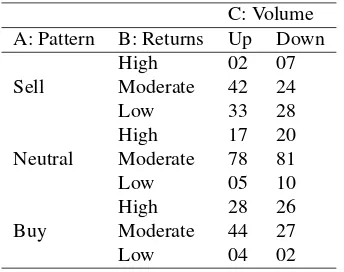
Table 3.3-dim Frequency table of 23 Nov 07 to 23 Nov 09
C: Volume A: Pattern B: Returns Up Down Sell
High 02 07
Moderate 42 24
Low 33 28
Neutral
High 17 20
Moderate 78 81
Low 05 10
Buy
High 28 26
Moderate 44 27
Low 04 02
These parameters are estimated by using their maximum likelihood estimators given below.
ˆ
λ0 =
1 IJ ∑ i ∑ j
ln(µij);
ˆ
λi =
1
J ∑
j
ln(µij)−λˆ0;
ˆ
λj =
1
I ∑
i
ln(µij)−λˆ0;
ˆ
λij = ln(µij)−
1
I ∑
i
ln(µij)−
1
J ∑
j
ln(µij)
+ 1 IJ ∑ i ∑ j
ln(µij),
To know more about log linear modeling and effect of levels of variables, see, Vijay (2011).
Log-linear modeling for 3-dimensional table: Log linear model for 3-dimensional contingency table is straight forward extension of (1), and is given by
ln(µijk) =λ0+λAi +λBj +λkC+λABij +λACik +λBCjk +λABCijk . (2) Maximum likelihood estimates of the parameters are also defined similarly. The above model is useful in explaining several interaction effects [Vellaisamy and Vijay (2007)], for example,
λABCijk =λABij = 0 (∀i, j, k) ⇔(A⊥B|C),
that is, A and B are independent given C. Similarly,
λABCijk =λ AB ij =λ
AC
ik = 0 (∀i, j, k) ⇔(A⊥B, C). All the hypotheses of independece/conditional independence for a 3-dimensional table are presented
below-H1: λABCijk =λ AC
ik = 0 (C⊥A|B);
H2: λABCijk =λ AB
ij = 0 (A⊥B |C);
H3: λABCijk =λ BC
jk = 0 (B⊥C|A);
H4: λABCijk =λ AC ik =λ
BC
jk = 0 (C⊥A, B);
H5: λABCijk =λ AB ij =λ
BC
jk = 0 (B⊥C, A);
H6: λABCijk =λ AB ij =λ
AC
ik = 0 (A⊥B, C);
H7: λABCijk =λ AC ik =λ
BC jk =λ
AB
[image:4.595.317.523.280.426.2]4
Analysis of contingency table
We consider 2-dimensional and 3-dimensional contin-gency tables for analysis. Chi-square test statistic is used to test whether a set of log-linear parameters is zero or equiva-lently, to test the hypotheses of independence. If any of the hypothesis of independence or conditional independence is rejected, the parameters will be used to analyze the influence of the categories of variables.
4.1
Analysis of 2-dimensional table
The 2-dimensional table of pattern and returns is created for daily returns of Maruti Sazuki Co, using the process given in Section-3. We use the closing price of stocks of the com-pany from 23 Nov 2007 to 23 Nov 2009 [Table-2]. We test the hypothesis of no association for this table by using
Z(H) = 2∗∑
i
∑
j
xij(ln(xij)−ln(µij)).
The Z(H) value is 182.634 which is greater thanχ2 0.95with
degree of freedom (4).
This leads to rejection of hypothesis of independence. That is, the variables A(Pattern) and B(Returns) are dependent on each other[Anderson (1996) pp 27-28].
We now obtain the maximum likelihood estimates of log lin-ear parameters. The main effect parameters are given in Table-4 and 5. The interaction parameter is presented in Table-6.
Table 4.Value ofλˆA
i for 2-dimensional table
ˆ
λA
i i=1 i=2 i=3 -0.1317 0.1367 -0.0051
Table 5.Value ofλˆB
j for 2-dimensional table
ˆ
λB
[image:5.595.357.507.311.410.2]j j=1 j=2 j=3 0.1038 0.7999 -0.9037
Table 6.Value ofλˆAB
ij for 2-dimensional table
ˆ
λABij j=1 j=2 j=3
i=1 -0.4550 0.1134 0.3417 i=2 0.0139 0.1169 0.1308 i=3 0.4411 -0.2303 -0.2109
Note that the parameterλˆAB1j andλˆAB2j attain the maximum value for j=3, that is, corresponding to Low returns. This implies that when the data exhibit selling pattern, there are more chances that the next return will be low in comparison to Medium and High. On the other hand,λˆAB
3j is maximum for j= 1 which shows that when the buying pattern is exhib-ited, there are more chances of the next return to be high. The main effectˆλA
i shows that the stock remain Neutral most of the time. λˆBj shows that the returns of the stock is main-tained at Moderate returns. Similarly, one can interpret the other values of interaction parameters.
4.2
Analysis of 3-dimensional table
We consider the returns for two different periods.4.2.1 The analysis for returns for the period 23 Nov 2007 to 23 Nov 2009
We now divide the data given in above table as per the intensity of volume, that is, Up and Down. This creates a 3-dimensional Table-3 for volume of transactions (Up, Down), pattern and returns. We test the seven hypotheses, given in Section-3, by using the test statistic
Z(H) = 2∗∑
i
∑
j
∑
k
xijk(ln(xijk)−ln(µijk)).
The following table presents the value of test statistic and standard chi-square value to test it at 95% level of signifi-cance.
Table 7.Hypothesis and Z(H) value table of 23 Nov07 to 23 Nov09
Hypo Z(H) Value Df χ20.95
H1 11.312 6 12.592
H2 132.384 6 12.592
H3 8.843 8 15.507
H4 13.546 10 18.307
H5 134.618 10 18.307
H6 137.087 8 15.507
H7 139.321 12 21.026
Clearly, H1, H3 andH4 cannot be rejected. This shows
that the volume is independent of pattern and returns. Under
H1, H3 andH4 the model contains the following non zero
parameters:ˆλAB
ij ,λˆAi ,λˆBj andˆλCk.The Maximum likelihood estimates for these parameters are shown in following tables.
Table 8.Value ofˆλA
i for 3-dimensional table
ˆ
λAi i=1 i=2 i=3
-0.0356 0.1170 -0.0815
Table 9.Value ofˆλB
j for 3-dimensional table
ˆ
λBj j=1 j=2 j=3
-0.1315 0.4250 -0.2935
Table 10.Value ofˆλC
k for 3-dimensional table
ˆ
λC
[image:5.595.97.258.607.670.2]k k=1 k=2 -0.004 0.004
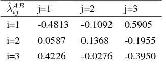
Table 11.Value ofλˆAB
ij for 3-dimensional table
ˆ
λAB
[image:5.595.352.515.746.809.2]Table-11 exhibits a pattern similar to that of Table-6. These estimated values of log-linear parameters can be interpreted similarly.
4.2.2 Data between Jan 2009- May 2009
[image:6.595.82.247.208.344.2]Again, we take same company data but different period. We now create a similar 3-dimensional table for the period of Jan 2009 to May 2009. The contingency table is given below:
Table 12.3-dim frequency table of Jan 09- May 09
C: Volume A: Pattern B: Returns High Low Sell
High 3 4
Moderate 7 18
Low 7 6
Neutral
High 3 2
Moderate 6 6
Low 2 1
Buy
High 9 11
Moderate 6 10
Low 2 2
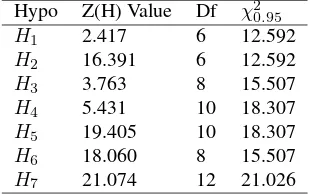
Table-12 of test statistic with respect to the hypotheses suggests that hypothesesH1,H3andH4 cannot be rejected
[image:6.595.86.241.438.535.2]at 95%level of significance. The non-zero interaction param-eters are estimated and given in the below tables:
Table 13.Hypotheses and Z(H) value table of Jan 09- Mar 09
Hypo Z(H) Value Df χ2 0.95
H1 2.417 6 12.592
H2 16.391 6 12.592
H3 3.763 8 15.507
H4 5.431 10 18.307
H5 19.405 10 18.307
H6 18.060 8 15.507
[image:6.595.90.237.583.614.2]H7 21.074 12 21.026
Table 14.Value ofλˆA
i for 3-dimensional table
ˆ
λAi i=1 i=2 i=3
0.1609 0.0248 -0.1857
Table 15.Value ofˆλB
j for 3-dimensional table
ˆ
λB
j j=1 j=2 j=3 0.0025 0.2662 -0.2687
Table 16.Value ofˆλC
k for 3-dimensional table
ˆ
λC
k k=1 k=2 0.00005 -0.00005
Once again the tables of parameters exhibit similar pattern, that is, when the pattern is Sell, there are more chances of return being low. For this data we get similar results.
Table 17.Value ofλˆAB
ij for 3-dimensional table
ˆ
λAB
ij j=1 j=2 j=3 i=1 -0.2634 -0.0165 0.2799 i=2 -0.0527 0.0727 -0.0200 i=3 0.3161 -0.0562 -0.2599
5
Conclusion and future aspect
We analyze the relationships among pattern, returns and volume of transactions of stock market data. The data is pre-sented in the from of contingency tables. These tables are analyzed by using log-linear modeling and the hypotheses of interactions are tested by using chi-square test statistic. We use these tables for further analysis to see the strength of re-lationship among the variables by using the maximum like-lihood estimates of various parameters of interaction. The Maruti-Sazuki Co. stock data clearly shows that pattern and returns are independent of the volume of transactions. Also, the log-linear model parameters show that the influence of categories of each of these variables will not depend upon the categories of other variables uniformly. The selling pat-tern and low value of next day return have more correlation than the other categories. Also, this analysis is not affected by Turn of the year effect.
One can similarly include more variables to analyze the multi-dimensional contingency tables. The construction of categories can also be defined by using other technical indi-cators, such as relative strength index, principal volume os-cillator etc. These tables may be further expanded to include more categories of each of the variables, for example, we have included two categories of volume and similarly three categories of other two variables.
Acknowledgements
Second author is thankful to the ministry of human re-sources and development (MHRD) for the fellowship grant. We thank the institute, IIT Jodhpur, for providing all the re-quired facilities. We are also thankful to the referees for their valuable inputs to strengthen the paper.
REFERENCES
[1] Anderson, E. B. (1996). Introduction to the Statistical Analysis of Categorical Data. Springer, New York. [2] Bollinger, J. (2002). Bollinger on Bollinger Bands.
McGraw-Hill, ISBN 0-07-127368-3.
[3] Boulesteix, A.L. (2006). Maximally Selected Chi-squared Statistics for Ordinal Variables. Biometrical Journal48, 451 - 462.
[4] Brad, M. B. and Odean, T. (2008). All That Glitters: The Effect of Attention and News on the Buying Behaviour of Individual and Institutional Investors.The Review of Financial Studies, 21(2), 785-818.
[6] Kateri, M. (2014).Contingency Table Analysis: Method and Implementation Using R,Birkh¨auser.
[7] Slavkovic A. B. (2006).Analysis of Discrete Data. Lec-ture Notes, Pennsylvania State University
[8] Vellaisamy, P. and Vijay, V. (2007). Some Collapsi-bility Results for N-Dimensional Contingency Tables.
Ann.Inst.Statist.Math, 59, 557 - 576.
[9] Vijay, V. (2011). Relationships Between Full and Layer Models With Applications to Level Merging. Communi-cations in Statistics-Theory and Methods, 40(4), 745 -761.
[10] Vijay, V. and Paul, P. (2015). A New Trading Band for Prediction of Buy and Sell Signals and Forecasting of States.International Journal of Applied Management Sciences and Engineering, 2(2), 34-54.