Conjugacy and subgroups of word hyperbolic groups

(1)

A Thesis Submitted for the Degree of PhD at the University of Warwick

http://go.warwick.ac.uk/wrap/3631

This thesis is made available online and is protected by original copyright. Please scroll down to view the document itself.

(2)

Conjugacy and Subgroups of

Word-Hyperbolic Groups

David John Buckley

A thesis submitted in fulfilment of the requirements for the degree of Doctor of Philosophy

Mathematics Institute, University of Warwick

(3)

(4)

List of Figures

1.1 A thin triangle, and a 3-correspondance . . . 8

2.1 Cutting across a long quasigeodesic . . . 27

2.2 A geodesic quadrilateral . . . 32

2.3 A thin part of a quadrilateral . . . 32

2.4 Points after the meeting points are distant . . . 32

2.5 A midpoint on a geodesic triangle . . . 45

2.6 Extending c. . . . 48

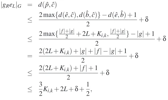
2.7 Bounding gReL . . . 51

3.1 Extending a long minimal coset representative . . . 65

3.2 Finding a shortcut over a minimal conjugate u . . . . 68

3.3 A large power of x . . . 69

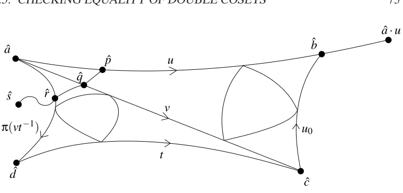
3.4 The double coset representatives . . . 75

3.5 The double coset representatives . . . 77

3.6 Finding a shorter h and k . . . . 78

4.1 The 1-balls around H and Ha are equal but not isomorphic . . . . . 85

4.2 A general triangle inΓ′ . . . 89

4.3 A hexagon inΓwhich maps to the triangle inΓ′ . . . 89

4.4 No point on[aˆ,ˆb]can chain-correspond only to a point on[aˆ′,eˆ′] . . 90

4.5 Vertices on[aˆ,eˆ]are equal to vertices on[aˆ′,eˆ′]after applying f . . . 91

4.6 In this situation, the dashed path must be longer than d(aˆ′,sˆ) . . . . 92

4.7 Again, the dashed paths cannot be too short . . . 93

4.8 The construction used in Case 4 . . . 94

4.9 A segment of a non-hyperbolic graph . . . 96

4.10 A loop u close to H . . . . 99

(7)

4.12 Geodesic triangle constructed outside of BK−1(ˆb) . . . 106

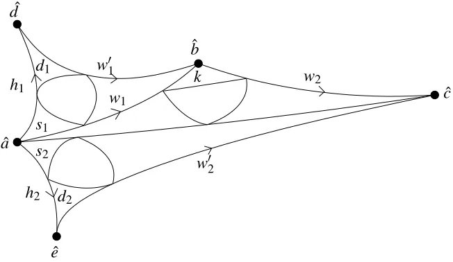
5.1 (1,k)-quasigeodesics lie close to geodesics . . . 110

5.2 (1,k)-quasigeodesic triangles are thin . . . 111

5.3 Removing loops from corners (left), and the first case of Proposition 5.2.1 (right) . . . 114 5.4 The second case of Proposition 5.2.1 . . . 117 5.5 A triangle inΓ′mapped intoΓ . . . 119

(8)

I would like to thank everyone who has helped me out during my time working on this thesis. This includes the various student societies of which I have been a part (particularly CompSoc, whose IRC service has allowed me to have many discus-sions both related to and completely unrelated to my studies!), the many graduate students and staff who have put up with me in the departmental common room, ev-eryone I have lived with and my family. The many undergraduates I have taught also deserve a mention for their patience with my somewhat strict marking, and their keeping me on my toes with respect to many mathematical fundamentals which might otherwise have grown somewhat hazy.

Particular thanks go to Dr Daan Krammer and Prof. Brian Bowditch for their input on my work, and of course my supervisor Prof. Derek Holt who introduced me to many of the problems dealt with in this thesis, and whose patience in finding mistakes and omissions in my proofs has been stellar.

Further, I would like to specifically thank my mother and sister, whose help in typing up my work has been a great help in allowing me to continue to use my hands.

My Ph.D. has been generously funded by the Engineering and Physical Sciences Research Council.

This thesis has been created using entirely open-source software including De-bian GNU/Linux, xfig, LA_{TEX and vim.}

Declaration

I declare that, to the best of my knowledge, the material contained in this thesis is original and my own work except where otherwise indicated, cited, or commonly known.

The material in this thesis is submitted to the University of Warwick for the degree of Doctor of Philosophy, and has not been submitted to any other university or for any other degree.

(9)

This thesis describes a number of algorithms and properties relating to Gromov’s word-hyperbolic groups. A fuller outline of the thesis is given, and a number of basic concepts relating to metric spaces, hyperbolicity and automaticity are first briefly detailed in Chapter 1. Chapter 2 then details a solution to the conjugacy problem for lists of elements in a word-hyperbolic group which can be run in linear time; this is an improvement on a quadratic time algorithm for lists which con-tain an infinite order element. Chapter 3 provides a number of further results and algorithms which build upon this result to efficiently solve problems relating to qua-siconvex subgroups of word-hyperbolic groups – specifically, the problem of testing if an element conjugates into a quasiconvex subgroup, and testing equality of dou-ble cosets. In Chapter 4, a number of properties of certain coset Cayley graphs are studied, in particular showing that graph morphisms which preserve edge labels and directions and map a quasiconvex subset to a single point also preserve a variety of other properties, for instance hyperbolicity. Finally, Chapter 5 gives a proof that all word-hyperbolic groups are 14-hyperbolic with respect to some generating set.

(10)

Below is a summary of notation used throughout the thesis. This notation is ex-plained more verbosely in the introduction.

Symbol Denotes

1 The identity element of a group.

d(x,y) The distance operator in a metric space.

(x,y)z The hyperbolic inner product, d(z,x)+d(z₂,y)−d(x,y).

ˆ

a_→w The path in an X -graph starting at ˆa and labelled by w.

ˆ

a_·w The vertex at the end of ˆa_→w.

∆(u,v) For words u and v, the inner product(aˆ_·u,aˆ_·v)aˆ.

d_γ(x,y) The length of the subpath of a pathγbetween points x and y.

[x,y] A path between points x and y.

X∗ The set of words with letters in a set X .

X±1 The set of elements of a set X along with their symbolic in-verses.

|w_| The length of a word or path.

|w_|G The length of the shortest word representing the same element

of G as w.

w−1 The symbolic inverse of a word or the reversal of a path.

wu For a word u, the word u−1wu.

wn For an integer i, the word formed by concatenating n copies of a word w.

w(i) The initial subword of a word w of length i.

w(i : j) The subword of a word w which skips the initial i letters and ends at the jth letter.

w[i] The ith letter of a word w.

wL The word w(

j

|w|

2

k

).

wR The word w(

j_|_w_|

2

k

:_|w_|).

wC The word wRwL.

w∞(i) The word wi(i), or wi(₋i)if i is negative.

(11)

passing through the base point.

O(f(n)) Computational complexity f(n), ignoring contributions from fixed structures.

A-FSA A finite state automaton which recognises words in A∗.

A-DFA A deterministic A-FSA.

x=yz Shorthand for_|x₋z_{| ≤}y.

u=Gv Words u and v represent the same group element. u=F v Words u and v represent the same free group element.

π(w) The short-lex reduction of a word w.

(12)

Chapter 1 Introduction

The concept of a word-hyperbolic group was explored by Gromov in [12] where he brought much previous work in the area together using some definitions involving groups with left-invariant hyperbolic metrics, the word-hyperbolic case of which will be given later. He shows among other things that in some sense “most” finite presentations define word-hyperbolic groups and that certain types of small cancel-lation group are word-hyperbolic.

It turns out that word-hyperbolic groups admit simple solutions to the first two problems outlined by Dehn in [5] for finitely presented groups G generated by a set

X :

The word problem: Given a word w_∈(X±1)∗, determine if w represents the identity element of G.

The conjugacy problem: Given words u,v∈(X±1)∗, determine if u and v are

conjugate elements of G.

In fact, there is a solution to a problem which generalises both of these in the torsion-free word-hyperbolic case, that of deciding whether a system of equations over elements in such a group admits a solution. This result is due to Sela in [22], although more general statements have since been proved.

An efficient solution to the word problem due to Shapiro is stated in Section 1.5, and a solution to the conjugacy problem is the topic of Chapter 2.

The third problem proposed by Dehn, the isomorphism problem of determin-ing whether two such groups are isomorphic has also been shown to be solvable at least for torsion free word-hyperbolic groups. Sela first showed in [21] that this is

(13)

solvable for torsion free word-hyperbolic groups with no essential small action on a real-tree and he has an unpublished proof for arbitrary torsion-free word-hyperbolic groups; Dahmani and Groves proved in [4] that the problem is solvable in the more general class of torsion free relatively hyperbolic groups with abelian parabolics (a class which in particular includes torsion free word-hyperbolic groups).

All three of these problems are known to admit no solution in the setting of general finitely presented groups.

The reader may notice that torsion in word-hyperbolic groups appears to lead to complications which are often hard to work with. The isomorphism problem for arbitrary word-hyperbolic groups remains open at the time of writing, and torsion plays a part in complicating some of the proofs given in this thesis.

In Chapter 2 we present a solution to the conjugacy problem for finite lists of elements of an arbitrary word-hyperbolic group which will run in time O(mµ)where

m is the number of words in each list and µ is an upper bound on the length of

said words. This is an improvement upon a quadratic time algorithm for lists which contain an infinite order element given in [3] - and an exponential time algorithm for lists of torsion elements outlined in the same paper. Our solution will in fact produce a complete description of the set of all conjugating elements, and in particular the centraliser of a given list of elements.

In Chapter 3 we show that given a quasiconvex subgroup H of a word-hyperbolic group, there is an algorithm which checks whether an input word represents a con-jugate of an element of H, and again, this algorithm will run in linear time if both the group and the subgroup are held constant. We also show that it is possible, again in linear time, to test if two double cosets HuK and HvK are equal for quasiconvex subgroups H and K, provided H and K are held constant.

Chapter 4 expands upon some work by Foord in [9], and gives some properties of certain coset Cayley graphs of subgroups of word-hyperbolic groups, specifically giving some bounds on hyperbolicity and the distance from the base point before which they become “eventually homogeneous” in the torsion free case, going on to show some simple facts about words which label geodesics distant from the base point.

Finally, in Chapter 5 we present a proof that there is a upper bound on the

mini-mum constant of hyperbolicity of a word-hyperbolic group over all finite generating

(14)

The rest of this chapter outlines the definitions which will apply during the rest of the thesis.

1.1 A Note on Computational Complexity

A number of results in the thesis make reference to running times of algorithms. These are normally stated in terms of a number of “fixed” entities, for instance some word-hyperbolic group. Where a quantity is described as being in O(n)for some n, any part of the runtime which depends on these fixed entities is ignored: we presume that there is some constant K depending only on the fixed entities such that the runtime is O(Kn).

Unless noted otherwise, we will assume that the algorithms in question are to be run under a RAM model of computing; that is, one in which seeking to arbitrary

locations of memory and basic arithmetic can be performed in constant time. This is a sensible model for any algorithm being implemented upon modern computers provided the input is small enough that processing it will not exhaust the system

RAM.

The run-time of the algorithms detailed here appears to be unchanged when they are run on a Turing machine, provided the machine is given a sufficiently large num-ber of states, symbols, heads and tapes (the numnum-ber of states, symbols, heads and tapes will be dependent only on the ambient groups picked, however) and provided one is rather more careful in cases where it appears arithmetic is needed to be per-formed. We use a RAM model in the text to avoid having to repeatedly deal with these technicalities.

1.2 Metric Spaces and Paths

We assume the reader has at least a basic understanding of metric spaces.

Definition 1.2.1. LetΓbe a metric space.

A path α in Γis a natural (ie. arc length) parametrizationα:[0,l]→Γ of a

rectifiable curve inΓ. We will write x_∈αto denote that x lies in the image ofα. If

(15)

A two-way infinite pathαin Γis defined in the same way, except thatα maps fromR_{instead of an interval.}

A subpathα′of a (finite or two-way infinite) pathα is any restriction ofαto a bounded subinterval of its domain, ie.α_|_[_a_,_b_], reparametrised so thatα′(0) =α(a).

The reversal α−1:[0,l]→Γ of a path α is the map which sends t ∈[0,l] to

α(l₋t).

For points x,y∈Γ, we will often pick a specific pathα:[0,l]→Γbetween x and

y, ie. withα(0) =x andα(l) =y. Where such a path has been explicitly picked, we will write[x,y]as a shorthand.

Further, when such a path has been picked, suppose that c=α(a)and d=α(b)

for 0_≤a_≤b_≤l. We will write[c,d]to refer to the subpathα|_[_a_,_b_]between c and d,

and define d_α(c,d) =b−a. Often we will simply pick the points c and d to construct

such a path. Whenever this is done, we are implicitly picking values a and b in[0,l]

so that this operation is well defined even whenαis not injective.

We are now in a position to define a number of concepts relating to shortest paths.

Definition 1.2.2. Supposeαis a path in some metric spaceΓ.

For anyλ_≥1 andε_≥0, we define αto be a(λ,ε)-quasigeodesic if given any

subpath[a,b]ofαwe have d_α(a,b)_≤λd(α(a),α(b)) +ε.

αis a geodesic if it is a(1,0)-quasigeodesic (that is, an isometry). A geodesic

metric space is a metric space in which every pair of points in the space have a

geodesic connecting them.

For L>0 define αto have a property L-locally if every length L subpath of α

has that property. So for example, L-local quasigeodesics are paths for which each length L subpath is a quasigeodesic.

Finally, a two-way infinite path has one of the above properties if every bounded subpath does. Thus we may describe an infinite path as a quasigeodesic and so on.

1.3 X -graphs

(16)

The metric spaces which are dealt with in this thesis will all be labelled directed graphs, where the labels obey the criteria below.

Definition 1.3.1. SupposeΓis a directed graph which is connected ignoring edge directions, and has all edges labelled by elements of some finite set X . ThenΓis an X -graph if, for each vertex ˆp_∈Γand each x_∈X , there are unique edges e and f labelled by x, so that e starts at ˆp and f terminates at ˆp. An X -graph will always be endowed with a distinguished base vertex.

Thus, an X -graph is a pointed labelled directed graph in which any word whose letters are in X_∪X−1defines an edge path starting from any vertex, formalised as follows:

Definition 1.3.2. For a finite set A, let Anbe the set of tuples(a1, . . . ,an)where each ai∈A. We define the set A∗=S∞n=0An and write elements of A∗ without brackets and commas, that is, in the form a1a2···an. If u,v∈ A∗ we define uv to be the element of A∗defined by the concatenation of these strings.

Suppose X is a finite set. Define X±1to be the union of X with the set_{x−1: x_∈

X_}where x−1is assumed to never be an element of X .

An X -word is an element of(X±1)∗. We will normally have a fixed set X ; where this is the case, unless specified otherwise we will often simply describe an X -word as a word.

We define (x−1)−1 _{to be just x for any x}_∈_{X and then define} ₍_a

1···an)−1 = a−_n1_···a−₁1for any X -word a1···an. An X -word is reduced if it contains no subword of the form xx−1or x−1x where x_∈X .

Given a vertex ˆp in an X -graph Γ, and some x_∈X , let ˆp_·x be the terminal vertex of the edge labelled x which starts at ˆp, and let ˆp_·x−1be the initial vertex of the edge labelled x which ends at ˆp.

For any X -word w=a1···anthere is thus defined a unique vertex ˆp·w= (. . .(w· a1)·a2. . .)·an, and a unique path ˆp

w

→:[0,n]→Γlabelled by w which picks each

intermediate vertex and edge in the obvious way.

(17)

Given a group G generated by a set X , the Cayley graph of G with respect to X has vertex set G and edges connecting g to gx with label x for each g_∈G and x_∈X .

This is an X -graph, and the base vertex in this case will be taken to be the vertex representing the identity of G.

Similarly, the coset Cayley graph (sometimes called a Schreier diagram or rela-tive Cayley graph) of a subgroup H_≤G with respect to X has vertex set V =_{Hg : g_∈G_}(ie. the set of right cosets of H), and edges connnecting Hg to Hgx for each

Hg_∈V and x_∈X . Again, this is an X -graph, and we take the base vertex to be the

vertex representing the trivial coset H.

In fact, any X -graph Γ is just a coset Cayley graph of a subgroup of the free group on X . To see this, let ˆp be the base vertex of Γ. Let G be the free group generated by X with elements represented by reduced X -words, and let H be the set of reduced X -words w such that ˆp_·w=p. Then H is a subgroup of G whose cosetˆ Cayley graph with respect to X isΓ. In this construction, ˆp is the vertex representing

the trivial coset H. Much of Chapter 4 could therefore be equivalently restated in terms of coset Cayley graphs.

Definition 1.3.3. If ˆp is a vertex in an X -graphΓ and k_≥0, the k-ball around ˆp, or BΓ_k(pˆ), is the set containing all vertices ˆq with d(qˆ,pˆ)≤k. The superscript will

often be omitted where the X -graph is clear from the vertex.

Later on, we will often use the concept of a mid-vertex of a geodesic path in a graph. We define this now.

Definition 1.3.4. Suppose ˆx and ˆy are vertices in some graphΓ, and[xˆ,yˆ]is some

geodesic path connecting them. Let ˆp be some vertex on[xˆ,yˆ]such that|d(pˆ,xˆ)−

d(pˆ,yˆ)| ≤1. Then we say ˆp is a mid-vertex of[xˆ,yˆ].

Note that if the distance between two vertices is even, there will be one mid-vertex; if it is odd there will be two.

1.4 More about X -words

(18)

Suppose G is a finitely generated group. We will use the notation=G to

repre-sent equality of elements of G, and simply=to represent equality of words. When we wish to represent equality of words allowing cancellation of letters with their inverses (ie. under the free group), we will write=F.

Definition 1.4.1. Suppose w=a1a2. . .akis some X -word.

Denote the length, k, of w as_|w_|, and if G is a group generated by X then denote by_|w_|Gthe smallest length of an X -word equal in G to w.

Let w(i):=a1a2. . .aifor 0≤i≤ |w|. If i<0 let w(i)be the empty word and if i>|w|let w(i):=w.

This definition can be extended to the integers by considering w(i)to be a sub-word of wn or w−n for large enough n. In order to avoid confusion, we use w∞ to represent this extension in the following notation: if i_∈N_{and n}₌

j

i

|w|

k

then

w∞(i) =wnw(i₋n_|w_|), and if₋i_∈N_{, w}∞₍_i_{) = (}_w−1₎∞₍₋_i₎_.

WhereΓis an X -graph with base point ˆa, define the two-way infinite pathwf∞: R_→Γ _{by setting} _wf∞₍_i₎_:₌_a_ˆ_·_w∞₍_i₎ _{for any integer i and extending to} R _{in the}

obvious way.

Next, for 0_≤i_≤ j_≤k we let w(i : j):=ai+1. . .aj=Fw(i)−1w(j). Let w[i]:=ai. If f =j|w₂|k, we define wL :=w(f), wR:=w(f :_|w_|)and wC:=wRwL.

Note that if w labels a geodesic path in Γ then wL labels a path to a

mid-vertex and w=wLwR always. As an example, let w =abcde. Then w∞(11) = abcdeabcdea, w∞(₋3) =w−1(3) =e−1d−1c−1, wL=w(2) =ab, wR=w(2 : 5) = cde and wC=cdeab.

We can now define a “straight” word.

Definition 1.4.2. Given an X -graphΓand with base vertex ˆa, a non-empty word w is straight ifwf∞is a geodesic.

By fixing some ordering on X±1 we can produce a lexicographic ordering on X -words. We say w is a short-lex least representative if w labels a geodesic at ˆa and no other geodesic connecting ˆa to ˆa_·w has a label lexicocgraphically less than w.

(19)

y

z x

cz q

[image:19.595.104.433.88.206.2]

p cy cx

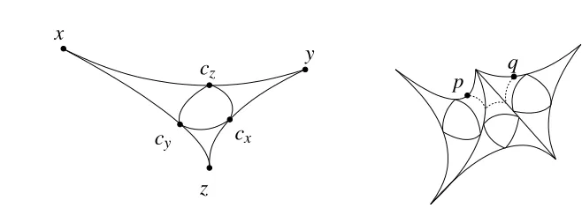
Figure 1.1: A thin triangle, and a 3-correspondance

Those definitions above which relate to the base point will only be used in the case whereΓis the Cayley graph of a group. As Cayley graphs are homogenous, they are therefore independent of the base point chosen.

1.5 Hyperbolicity

There are a number of equivalent definitions of hyperbolicity of a given space, many of which are for example given in [2] or [1]. The definition we will be using is that of having thin triangles.

Definition 1.5.1. LetΓbe a geodesic metric space.

For points x,y,z∈Γ, define the hyperbolic inner product

(x,y)z=

d(x,z) +d(y,z)₋d(x,y)

2 .

Given three points x,y,z_∈Γ, we define a triangle to be a choice of paths[x,y],

[y,z]and[z,x]. We say the triangle is geodesic (resp. quasigeodesic, local geodesic,

. . . ) if each of the three paths which make it up are geodesic (resp. quasigeodesic, . . . ).

On a triangle connecting these three points, define the meeting point on the side

[x,y]to be the point cz ∈[x,y]such that

d_[_x_,_y_](x,cz) =

d_[_x,y](x,y) +d[x,z](x,z)−d[y,z](y,z)

2 .

(20)

and cy similarly as in Figure 1.1. Note that in the case of a geodesic triangle, d(x,cz) = (y,z)x.

Suppose that p is a point on [x,cz]. We say the point q ∈ [x,cy] such that d_[_x_,_c_y_](x,q) =d_[_x_,_c_z_](x,p) corresponds to p and vice versa. By relabelling the

cor-ners, we may find a corresponding point to each point on each of the three sides of the triangle. Observe that the meeting points all correspond to each other and hence have two corresponding points (except in degenerate cases where the meeting points are equal), and that all other points have one corresponding point (except in similar degenerate cases).

The triangle isδ-thin if d(p,q)≤δfor all such corresponding points p and q.

It isδ-vertex-thin if d(pˆ,qˆ)≤δfor all corresponding vertices ˆp and ˆq.

A geodesic space is δ-hyperbolic if all geodesic triangles in it are δ-thin. A graph isδ-vertex-hyperbolic if every geodesic triangle in the graph whose corners lie on vertices is δ-vertex-thin and δ is an integer. In either case we will assume

δ≥1 to avoid complications in run times and so on.

A finitely generated group G=<X> is δ-hyperbolic with respect to X if its

Cayley graph with respect to X isδ-hyperbolic.

In a construction involving many triangles sharing common sides, we will use the phrase p n-corresponds to q if there is a sequence p=r0,r1,r2,···,rn=q of points such that ricorresponds (via a previously constructed triangle) to ri+1for all i. More generally, we will say that points chain-correspond if there exists an n_∈N

such that they n-correspond. This is illustrated on the right hand side of Figure 1.1.

Notice that for any points x,y,z∈Γwe have(x,z)y+ (y,z)x=d(x,y). This fact

is used in many places to produce bounds on d(x,y).

For an X -graph Γ with base vertex ˆa, if we have X -words u,v which label

geodesics at ˆa then the value of (aˆ_·u,aˆ·v)aˆ in some sense measures the amount

of cancellation in the word u−1v when it defines a path starting at ˆa_·u. When

Γ is a Cayley graph, notice that (aˆ_·u,aˆ·v)aˆ = |u|G+|v|G−|uv −1_|G

2 is independent of

the specific vertex ˆa. Thus, when some group G has been picked, we will write

∆(u,v) = (aˆ·u,aˆ·v)aˆ.

(21)

with words – that is, labels of paths which connect vertices. Most of the literature, however, uses the hyperbolicity constant rather than vertex-hyperbolicity constant, so we will for the most part be using this constant also to simplify the use of results from elsewhere.

The property of being δ-hyperbolic for some δis a property of the group and not just the generating set (see [12]), although the particular value ofδwill likely change depending on the particular generating set used.

Of course, knowing that such a constantδexists is not particularly helpful for writing explicit algorithms which will often use the value ofδ. In [7] an algorithm is given (and in fact implemented in D. F. Holt’s KBMAG package) which can, given a finite presentation for a word-hyperbolic group, compute such a constant. In fact, the algorithm computes the minimum vertex-hyperbolicity constant for the Cayley graph relative to the given generating set.

This algorithm terminates if and only if the presentation defines a word-hyperbolic group, and has no bound on its running time: It is impossible to predict when the algorithm will complete, only that it will at some point do so. We will therefore assume that for any word-hyperbolic group mentioned in this thesis, the algorithm has already been executed and thus the constantδis known.

Note that this indeterminate runtime is the best that we can hope for. Given a δ-hyperbolic group, it is rather easy to test if that group is trivial: use the solution of the word problem to show that each generator is equal to the identity. In fact, the trivial group is 1-hyperbolic with respect to any generating set. If there were

an efficient algorithm which determined whether or not a given presentation was hyperbolic, it would therefore be able to determine whether or not a given finite presentation is a presentation of the trivial group. This is well known to be impos-sible.

We noted earlier that the word problem was solvable in the setting of word-hyperbolic groups. In [8] a solution to the word problem due to Shapiro is given which runs in linear time on a Turing machine with two tapes, as follows.

Lemma 1.5.2. Suppose that G is aδ-hyperbolic group. Then there is an algorithm which, given a word w in the generators of G will return the short-lex least repre-sentative of w in time O(_|w_|).

(22)

by π operating on elements, words and lists of elements or words in the obvious way. Of course, we will also use it implicitly, since it implies that operations like finding the length_|g_|Gof an element g, or deciding equality of two elements can be

performed in time linear in the length of the input words.

1.6 FSAs, DFAs and Automatic Groups

Another class of finitely generated groups which is of computational interest is the class of automatic groups, which are defined by certain finite state automata. A lot of detail in these definitions and results will be omitted; Chapter 13 of [14] gives a rather fuller outline of the theory of automatic groups and regular languages.

Definition 1.6.1. Given a set A, let A′=A_{∪ {}ε_}whereεis assumed not to be in A. A finite state automaton M on an alphabet A (or A-FSA) is a finite set S of states, a subset X _⊂S of start states, a subset Y _⊂S of accepting states and a set

τ_⊂S_×A′_×S of transitions.

The set of transitions allow us to regard M as a directed graph G with vertex set S and an edge connecting s to t with label a whenever(s,a,t)∈τ. An edge with

labelεis called anε-transition.

We say M is deterministic, or M is an A-DFA, if X has only a single element s0∈X , there are noε-transitions and for all s∈S and a∈A there is at most one edge in G labelled a which starts at s.

We say an element w_∈A∗ is accepted by M if there is a path in G starting at an element of X and ending at an element of Y whose label, after deleting all occurrences ofε, is w.

A subset of A∗ is called a language. The set of all words accepted by M is the language of M.

A language is regular if it is the language of an A-FSA.

In the deterministic case, notice that τ defines a partial function σ: S_×A_→ S. By adding a “reject” state r to S, we can make σ a full functionσ′ by setting σ′₍_s_,_a_{) =}_{r whenever} _σ′₍_s_,_a₎ _{is not defined. We can extend this to a transition}

functionσ: S_×A∗_→S by lettingσ(s,w):=σ′(σ′(σ′(s,a1),a2), . . . ,an)whenever w=a1a2···an∈A∗. Thus w is accepted if and only if σ(s0,w)∈Y , and one can

(23)

Every regular language is in fact accepted by a DFA. In section 13.1.6.1 of [14], for instance, a method is given to produce a DFA from any FSA.

A basic property of regular languages is that they obey the pumping lemma (see [15], Lemma 3.1 for example). A quick sketch proof is given here, as a similar technique is used in Section 2.3.1.

Proposition 1.6.2. Suppose M is an A-DFA. Then there is a constant K such that for any word w in the language of M with_|w_{| ≥}K there are words a,b,c∈A∗such

w=abc,_|b_|>0 and abnc is in the language of M for all n>0.

Proof. Let K be the number of states in M, let s0 be its start state and let σ be

its transition function. If _|w_{| ≥}K then when reading w, some state is hit twice,

ie. there is some state s with s=σ(s0,w(i)) =σ(s0,w(j)) for some i< j. Then

σ(s,w(i : j)) =s, so let a :=w(i), b :=w(i : j)and c :=w(j :|w|)and for any n≥0

we haveσ(s0,abnc) =σ(s0,abc) =σ(s0,w). In particular, abnc is also accepted by

M.

There are many other definitions of a regular language which are equivalent to this, for instance, regular expressions. We will not need these definitions, however, so we omit them. We do, however, make use of (synchronous) n-variable FSAs which we now define.

Definition 1.6.3. For this definition, given a set A, let A′=A_{∪ {}$_}where $ is some symbol which is not in A.

Given a tuple T = (w1, . . . ,wn)of words with letters in A, let l be the length of the longest word in T . For each i, let w′_i be wi with a string of $ symbols added onto the end so that each w′_i has length exactly l. Now let Te =a1_···al where aj:= (w′₁[j], . . . ,wn′[j])so thatT , the padding of T , is an element ofe (A′n)∗.

An n-variable A-FSA M is now defined to be simply an A′n-FSA. The language of M is the set of elements of(A∗)n_{which, after padding, are accepted by M.}

We say that a subset of(A∗)n _{is a regular n-variable language if it is the} lan-guage of an n-variable A-FSA.

(24)

Proposition 1.6.4. Suppose A is a finite set containing l elements.

(1) The empty set is the language of an A-DFA with 1 state.

(2) A∗is the language of an A-DFA with 1 state.

(3) For any word y_∈A∗, the set _{y_} is the language of an A-DFA with_|y_|+1

states.

(4) For any non-empty word y_∈A∗, the set_{yn: n_∈Z_,_n_≥₀_}_{is the language of}

an A-DFA with_|y_|states.

Now suppose that there are are n1-variable and n2-variable A-FSAs which have languages L1and L2, and have k1and k2states respectively.

(5) Projection of L1 to any its first factor is the language of an A-FSA with k1 states.

(6) L1×L2is the language of an n1+n2-variable A-FSA with k1k2states.

Suppose that n1=n2.

(7) L1∪L2is the language of an n1-variable A-FSA with k1+k2states.

(8) L1∩L2is the language of an n1-variable A-FSA with k1k2states.

Finally, suppose that n1=n2=1.

(9) _{(w,w): w∈L1}is the language of a 2-variable A-FSA with k1states.

(10) The concatenation L1L2 ={w1w2 : w1 ∈L1,w2 ∈L2} of L1 and L2 is the language of an A-FSA with k1+k2states.

All of the automata above can be computed in time O(l2s), where s is the number of states in the new automaton.

Proof. For (1) let S=X =Y =_{1_}and τbe the empty set. For (2), let S =X =

Y =_{1_}and letτ=S_×A′_×S.

(25)

For the remainder of the examples, assume the FSAs have state sets Si, start

states Xi, accept states Yiand transitionsτi. For convenience, assume that S1∩S2=

φ.

For (5) let S=S1, X =X1, Y =Y1andτ={(s,a1,t):(s,(a1, . . . ,an1),t)∈τ1},

replacing any transitions labelled $ with transitions labelledε.

For (6) if both automata have one variable, let S=S1_×S2, X =X1_×X2 and

Y =Y1_×Y2. Letτ′_i=τi∪ {(s,$,s): s∈Si}for each i and then let

τ=_{((s1,s2),(a1,a2),(t1,t2)):(s1,a1,t1)∈τ′1,(s2,a2,t2)∈τ′2}.

The multiple variable case is similar but requires that one be a little careful with transitions labelled $.

For (7) let S=S1∪S2, let X=X1∪X2and let Y =Y1∪Y2. Finally, letτ=τ1∪τ2.

For (8) let S=S1×S2, let X =X1×X2, let Y =Y1×Y2and letτ={(s1,s2,a,t1,t2):

(s1,a,t1)∈τ1,(s2,a,t2)∈τ2}.

For (9) let S=S1, X =X1, Y =Y1andτ={(s,(a,a),t):(s,a,t)∈τ1}.

For (10) let S=S1∪S2, X =X1 and Y =Y2and letτ=τ1∪τ2∪ {(y,ε,x): y∈ Y1,x∈X2}.

In each case, the sets S,X,Y and τ define the required automaton and can be

computed in the required time.

We now define various types of automatic groups.

Definition 1.6.5. Suppose that G is a group generated by a set X .

A language W _⊂(X±1)∗is a cross-section of G if each element of G is equal to at least one element of W . If W is regular, we say W is a regular cross-section of G.

Suppose that W is a regular cross-section of G. Let A be the set containing all of X±1as well as the identity in G.

If the set _{(u,v) _∈W2 : ux =G v} is a regular 2-variable language for each x_∈A then we say G is automatic with respect to W . A group is automatic if it is automatic with respect to some regular cross-section.

(26)

P. Papasoglu proved in [19] that a group is word-hyperbolic if and only if it is automatic with respect to the set W of all words labelling geodesics in the Cayley graph (that is, if the group is strongly geodesically automatic). In fact a word-hyperbolic group is automatic with respect to the set of short-lex least representa-tives of elements (this is Theorem 3.4.5 of [6]).

Word-hyperbolic groups are also conjugacy automatic with respect to the set of geodesic-labelling words (see Lemma 4.2 of [11] for a proof of this fact which uses the fact that word-hyperbolic groups are biautomatic with respect to the set of geodesics). Since the language of short-lex least representatives is regular and the intersection of two regular languages is regular, word-hyperbolic groups are conjugacy automatic with respect to the set of short-lex least representatives as well. In particular, for a word-hyperbolic group generated by a set X , there is an X±1 -DFA whose language is the set of all short-lex least words, the short-lex word

acceptor, and another X±1-DFA whose language is the set of words which la-bel geodesics in the group’s Cayley graph, the geodesic word acceptor. We will assume therefore that these automata have already been computed for any word-hyperbolic group we are given.

Much like with hyperbolicity, it is impossible to determine whether or not an arbitrary finitely presented group is automatic – in fact, the problem here is made even more difficult as one must search for a regular cross-section W , which might not be something easily described like the set of geodesic-labelling words.

1.7 Other Notation

We close this chapter with some other miscellaneous notation which is used through-out.

Many of the results in the thesis relate to conjugacy. We adopt a shorthand to express conjugation.

Definition 1.7.1. Supposing g,h∈G, we will denote conjugation of g by h using

superscripts, so that gh=h−1gh.

(27)

(28)

Chapter 2 The Conjugacy Problem for Lists

2.1 Introduction

In [3], Bridson and Howie give a solution of the conjugacy problem for finite lists

A= (a1, . . . ,am)and B= (b1, . . . ,bm)of elements in a word-hyperbolic group – in fact, they prove that the problem is solvable in time O(mµ2)for a torsion free group,

where µ is an upper bound on the length of elements in both lists.

The aim here is to both improve the bound on running time to O(mµ), and to tie up the rather limp conclusion in part 2 of Theorem B of [3], in which their algorithm simply terminates when the lists contain entirely elements of finite order without giving any results on the conjugacy.

The ideas used here closely relate to the ideas in [8], in which Epstein and Holt show that the conjugacy problem for single elements in a word-hyperbolic group can be solved in linear time if one assumes a RAM model of computing. They do so by showing that infinite order elements tend to be well-behaved when raised to large powers, and finite order elements can be conjugated to elements of short length whose conjugacy can be precomputed. In fact, we use a number of results

from that paper which relate to these facts in order to establish the result here.

We will presume for the duration of this chapter that the ambient finitely

gen-erated group G has been fixed along with a finite generating set X , and that G is δ-hyperbolic for someδwith respect to this generating set (we will assumeδis an integer andδ>0 to simplify some reasoning later on). All words in this chapter are

X -words, and all geometric constructions occur inside the Cayley graphΓof G with

(29)

respect to X , inside which we will assume that the vertex ˆe represents the identity

element of G.

We will also assume that an ordering on the generators has been picked, so that the notion of a short-lex least representative word for each element exists and that the short-lex word acceptor for G has been computed.

The technicalities behind the proof in the case where one element, say a1, has

infinite order are largely covered by solving the conjugacy problem ah₁=Gb1for h

as in [8]. In the process of doing so, we can find a useful description of elements of the centraliser C of a1 and then test if for some c∈C we have Ach =GB. Of

course C is infinite, so it is important to perform this testing efficiently. Section 2.3 describes a way of doing so.

Unfortunately, since we can only obtain this form of the centraliser for infi-nite order elements we run up against problems when we consider lists of torsion elements. It is, however, possible to show that provided we bound the number of el-ements in our lists, we can efficiently find a pair of lists A′and B′such that Ah=GB

if and only if A′h=GB′ and such that either A′or B′contains an infinite order

ele-ment, or each element in A′and B′is of bounded length for some element g. In the latter case, one may simply use the exponential algorithm given in [3] to finish the solution.

The disadvantage of computing in this way is that for lists with more elements,

the amount of computation required grows in at least exponential fashion. However, it can be shown that if there are sufficiently many finite order elements in the list then

its centraliser is finite. In particular, there are only a finite number of elements which can simultaneously conjugate the initial elements of one list to the initial elements of the other, so we need only test these centralising elements on the remainder of the elements of the lists to complete the procedure.

In fact, all of the methods we use above will produce a complete description of the set of all conjugating elements as a regular set. Thus we have:

Theorem 2.1.1. Given integers δ_≥1 and l, there is an algorithm which, given

a δ-hyperbolic group G=<X|R> with |X| ≤l, a number m≥0 and lists A=

(a1,···,am) and B= (b1,···,bm), each containing words in the generators of G, can find a (non-deterministic) X±1-FSA whose language L satisfies:

(30)

• for any g_∈G such that Ag=GB there is an element w∈L with w=Gg.

If _|ai_{| ≤}µ and_|bi_{| ≤}µ for each 1_≤i_≤m then the algorithm will run in time O(mµ). It can be modified to return a single conjugating element g_∈G with Ag=B,

if one exists, without affecting the running time.

Because the methods here express all conjugating elements, they additionally allow computation of the centraliser of a list of elements.

2.2 Notation

In this section, we provide some notation which is used during the remainder of the chapter. We start by suggesting that the reader familiarise themselves with the definitions in Section 1.4.

Next, recall Lemma 1.5.2, that we have a functionπwhich returns the short-lex least representative in G of any word and can be computed in time linear in input word length. We extendπto operate on lists and sets in the obvious way.

There are a number of constants which will be used throughout this chapter (as well as some points in later chapters where this chapter’s results are used). These are:

• L :=34δ+2

• V , the number of vertices in B2δ(eˆ)

• Q, the number of vertices in B₄_δ(eˆ) • M :=103δ2V3L2

2.3 The Infinite Order Case

In this section, we will assume that we are given two equal length lists A and B whose elements are X -words, and that all elements of A and B have length at most

µ. We will also assume that the first element of A is of infinite order.

The aim of the section is to test which elements g_∈ G have Ag =G B. The

(31)

We begin with several sections which bring together results from other sources and then put those results together to give an algorithm which finds elements which conjugate A to B.

2.3.1 Results From [8]

In [8] (Section 3), it’s proved that the conjugacy problem for single elements is linear in the total input element length. The proof has several steps. The first few will be followed here as well.

The first step is to show that elements that are “difficult to shorten” are actually of infinite order, and behave nicely when raised to large powers. This result is Lemma 3.1 of [8].

Proposition 2.3.1. Let w be some short-lex least word. Let u be the short-lex least representative of wC. If u has length strictly greater than 2L, then all positive powers of u label L-local(1,2δ)-quasigeodesics.

In Proposition 2.3 of [8] it is proved that such a local quasigeodesic lies close to a geodesic.

Proposition 2.3.2. If w is an L-local(1,2δ)quasigeodesic inΓ, and u is a geodesic

connecting its endpoints, then every point on w is within 4δof a point on u and vice versa. Also, if_|w_{| ≥}L then_|u_{| ≥} 7₁₇|w|.

In particular, if_|wC|>2L then w is of infinite order as there is no bound on the

length of shortest representatives of its powers. We will use this fact extensively in the next section also.

The next step is to show that such a word u can be equated with some root of a conjugate of a short-lex straight word. The following two results summarise Section 3.2 of [8].

Proposition 2.3.3. Suppose u is some short-lex least word such that all positive powers of u label L-local (1,2δ)-quasigeodesics and |u|>L. Then there exists

some integer 0<k≤Q2and some word a whose length is less than or equal to 4δ

such thatπ(a−1uka)is short-lex straight.

(32)

The second proposition can be proved in a similar way to the Pumping Lemma, Proposition 1.6.2. Repeatedly read u through the short-lex word acceptor until some state is hit for the second time after reading a complete copy of u. In this case, reading u again will just cycle over previous states so u must be short-lex straight.

Thus we have the following code to test for short-lex straight-ness:

Algorithm 2.3.5. Test if an X -word is short-lex straight

1: function TESTSLS(u)

Input: An X -word u.

Output: True if a is short-lex straight; false otherwise.

2: WA_←SHORTLEXWORDACCEPTOR(G)

3: S_←STATES(WA)

4: w_←u|S|

5: for s_∈S do

6: visited[s]_← f alse ⊲States hit after reading complete copies of u

7: end for

8: s_←STARTSTATE(WA)

9: f _←TRANSITIONFUNCTION(WA)

10: visited[s]_←true

11: for i :=1 to_|w_|do

12: s_← f(s,w[i])

13: if_¬ISACCEPTSTATE(WA,s) then

14: return false

15: end if

16: if i=0 mod_|u_|then

17: if visited[s]then

18: return true

19: end if

20: visited[s]_←true

21: end if

22: end for

23: end function

And we can find a short-lex straight power as follows:

(33)

1: function FINDSLSPOWER(a)

Input: An X -word a for whichfa∞is a L-local(1,2δ)quasigeodesic.

Output: An X -word h and an integer i withπ((ai)h₎_{short-lex straight.}

2: for h_∈B₄_δ(1)do ⊲Find straight power using Proposition 2.3.3

3: for i_{∈ {}1, . . . ,Q2}do

4: if TESTSLS(π(h−1aih)) then ⊲Must happen at least once

5: return h,i

6: end if

7: end for

8: end for

9: end function

Once a word is short-lex straight, it is easier to test conjugacy against it. The next result summarises Section 3.3 of [8].

Proposition 2.3.7. If u is short-lex straight and v is a word such thatfv∞is a(1,2δ)

L-local quasigeodesic with_|v_|G>L, and g−1vg=Gu for some g, then there exists a word h with_|h_{| ≤}6δsuch thatπ(h−1vh)is a cyclic conjugate of u.

One can test if a word u is a cyclic conjugate of another word v by testing if

v appears as a substring of u2, which can be done for instance using the Knuth-Morris-Pratt algorithm which runs in time1 O(_|u_|+_|v_|). We denote the use of this algorithm by FINDSUBSTRINGand later, FINDSECONDSUBSTRING.

The following pseudocode will test conjugacy of such words u, v:

Algorithm 2.3.8. Test if a short-lex straight word is conjugate to a “long” word.

1: function TESTCONJUGACYSLSLONG(u,v)

Input: A short-lex straight X -word u and an X -word v for whichfv∞is a L-local (1,2δ)quasigeodesic.

Output: An X -word g with ug=Gv or null if no such g exists.

2: for h_∈B₆_δ(1)do ⊲Test conjugacy using Proposition 2.3.7

3: i_←FINDSUBSTRING(u2,π(hvh−1))

1_{Strictly speaking, the standard KMP algorithm will run in worse than linear time on a Turing}

(34)

4: if i is not null then

5: return u(i)h

6: end if

7: end for

8: return null

9: end function

A refinement of the proof of the above statement gives a nice form for elements of the centraliser of a short-lex straight word. This result summarises Section 3.4 of [8].

Proposition 2.3.9. If z is short-lex straight and yl=z with l maximal, then g_∈CG(z) implies that g=Gyiy1h, with y1a prefix of y, i∈Zand|h| ≤2δ. Further, y1depends only on h.

l, y and the set of words y1h can be computed in time O(|z|).

Again, here is the algorithm in pseudocode:

Algorithm 2.3.10. Find a “nice” superset of the centraliser of a short-lex straight

word.

1: function FINDSLSCENTRALISERSUPERSET(z)

Input: A short-lex straight X -word z

Output: A short-lex straight word y with yl =z for some l and a set S with CG(z)⊂ {yns : n∈Z,s∈S}.

2: i_←FINDSECONDSUBSTRING(z2, z)

3: y_←z(i) 4: S_{← {}}

5: for h_∈B₂_δ(1)do ⊲Find centraliser of a using Proposition 2.3.9

6: i_←FINDSUBSTRING(z2,π(hzh−1)) 7: if i is not null then

8: S_←S_{∪ {}z(i)h_}

9: end if

10: end for

11: return y,S

(35)

Suppose that z=π(a−1(uC)ia)is short-lex straight, that yl =z with l maximal,

thatfv∞is an L-local (1,2δ)quasigeodesic, that b−1zb=Gvi and that g−1ug=Gv.

Note that

zb =G vi

=G (ui)g

=G (uCi)(uL) −1_g

=G za −1₍_u

L)−1g

so that a−1(uL)−1gb−1 ∈CG(z), and so is equal in G to yny1h where n is some

integer, h is a word of length at most 2δand y1is a prefix of y that depends only on h. Therefore g=GuLayny1hb.

This fact is used in the following algorithm which returns a word p of length

O(_|u_|), a short-lex straight word y of length O(_|u_|)and a set S of at most V words each of length O(_|u_|+_|v_|)such that if g−1ug=Gv then g=G pyns for some n∈Z

and some s_∈S.

Algorithm 2.3.11. Find a “nice” set of candidates for conjugating elements.

1: function GETCONJUGATIONCANDIDATESEH(u,v)

Input: Two X -words u and v which label geodesics inΓand have _|uC|G>2L

and_|vC|C>2L

Output: An X -word p, a short-lex straight word y and a set S with(up)i₌_yj_for

some i,j_∈Z_{and such that}π(_w₎_{∈ {}π(_pyn_s₎_{: n}_∈Z_,_s_∈_S_}_{whenever u}w₌_G_v.

2: a,i←FINDSLSPOWER(π(uC))

3: z_←π(a−1(uC)i_a₎

4: b_←TESTCONJUGACYSLSLONG(z,π((vC)i))

5: if b is null then

6: return 1,1,{}

7: end if

8: y,S←FINDSLSCENTRALISERSUPERSET(z) 9: return uLa,y,{sb(vL)−1: s∈S}

10: end function

(36)

2.3.2 Finding Long Powers of Infinite Order Elements

In this section, we will show that given an X -word w which represents an infinite

order element of G, we can find a short-lex reduced word w′which is conjugate in

G to a power of w and for whichπ(w′_C)is longer than 2L. Thus given two infinite order words u and v we may find conjugates of powers of u and v to which we may apply GETCONJUGATIONCANDIDATESEH.

We begin by recalling some well-known properties of word-hyperbolic groups and hyperbolic spaces; these results are taken from [1] although similar results ap-pear in many other expositions of the subject area. The exact values in the

state-ments are taken from the proofs in [1] (the statestate-ments generally simply state that the constants in question exist). The first is Proposition 3.2 of [1].

Proposition 2.3.12. For any X -word w which is of infinite order in G and labels a geodesic in Γ, the two way infinite path wf∞ in Γ is a(λ,ε)-quasigeodesic, where

λ=_|w_|V andε=2_|w_|2V2+2_|w_|V .

The next is Theorem 2.19 of [1].

Proposition 2.3.13. The function e :R_≥₀_→R_≥₀_{with e}₍₀_{) =}δ_{and e}₍_l_{) =}₂δl−2for l>0 is a divergence function for anyδ-hyperbolic space (ie. given geodesicsγ=

[x,y]andγ′= [x,z], if r,R∈N_{with r}₊_R_<_min_{|γ_|_,_|γ′_|}_{and d}(γ(_R₎_,γ′₍_R₎₎_>_e₍₀₎_,

ifαis a path fromγ(R+r)toγ′(R+r)lying outside the ball of radius R+r around x, then_|α_|>e(r)).

Finally, Proposition 3.3 of [1].

Proposition 2.3.14. In a hyperbolic space with divergence function e, given con-stants λ _≥ 1 and ε_≥ 0, there exists D = D(λ,ε,e) such that if α is an (λ,ε) -quasigeodesic andγis a geodesic starting and ending at the same points asαthen every point onγis within a distance D of a point onα. It suffices to take D satisfying e(D−₂e(0))_≥4D+6λD+ε.

We now use these results to find some power n of an infinite order word w such that_|(wn)C|Gis large. Recall M from Section 2.2.

(37)

Proof. By Proposition 2.3.13, the function e(0) =δ, e(l) =2δl−2for l>0 is a

diver-gence function forΓ. By Proposition 2.3.12 we see thatwf∞is a(λ,ε)-quasigeodesic

γ, whereλ=_|w_|V andε=2_|w_|2V2+2_|w_|V . The first aim is to find a suitable D for

Proposition 2.3.14.

Let D :=104δ2LV . Then

e

D₋δ

2

= 22Dδ− 5 2

= 1

4√2

e2Dδ log 2

,

but ex> x_3!3 > x₃3for any x>1, so noting that 3 log 2_≥2, we have

e

D₋δ

2

≥ 1

4√2

D

3_×2δ

3 log 2

≥ 1

4√2

D

6δ

2

and by substituting in D

e

D₋δ

2

≥ 1

4√2

104δLV

6

2

= 10

8

36_×4√2δ

2_L2_V2

≥ 480000δ2L2V2.

Recall that_|w_{| ≤}2L,λ=_|w_|V andε=2_|w_|2V2+2_|w_|V , so

e

D₋δ

2

≥ (12+12+12+12)104δ2L2V2

= 12_×104δ2L2V2+12_×104δ2L2V2+12_×104δ2L2V2+12_×104δ2L2V2

≥ 4_×104δ2LV+12LV_×104δ2LV+8L2V2+4LV ≥ 4_×104δ2LV+6_|w_|V_×104δ2LV+2_|w_|2V2+2_|w_|V

Conjugacy and subgroups of word hyperbolic groups

Conjugacy and Subgroups of

Word-Hyperbolic Groups

David John Buckley

Mathematics Institute, University of Warwick

Contents

List of Figures

Declaration

Chapter 1

Introduction

1.1

A Note on Computational Complexity

1.2

Metric Spaces and Paths

1.3

X -graphs

1.4

More about X -words

1.5

Hyperbolicity

1.6

FSAs, DFAs and Automatic Groups

1.7

Other Notation

Chapter 2

The Conjugacy Problem for Lists

2.1

Introduction

2.2

Notation

2.3

The Infinite Order Case

2.3.1

Results From [8]

2.3.2

Finding Long Powers of Infinite Order Elements