Some modified bifurcation problems with application to imperfection sensitivity in buckling

WITH APPLICATION TO IMPERFECTION SENSITIVITY IN BUCKLING

Thesis by

James Paul Keener

In Partial Fulfillment of the Requirements

For the Degree of Doctor of Philosophy

California Institute of Technology Pasadena, California 91109

1972

Acknowledgements

The author wishes to thank Professor Herbert B. Keller for making many helpful suggestions regarding the problems treated in this thesis. He has given freely of his time in offering ·advice, encouragement, and patient supervision throughout the course of this work.

The author is grateful to Mrs. Vivian Davies for her conscientious and painstaking typing of the manuscript.

The work represented by this thesis would have been con-siderably more difficult were it not for the constant love and encouragement of his wife Kristine,

to

Abstract

The branching theory of solutions of certain nonlinear elliptic partial differential equations is developed, when the non-linear term is perturbed from unforced to forced. We find

families of branching points and the associated nonisolated solutions which emanate from a bifurcation point of the unforced problem. ·Nontrivial solution branches are constructed which contain the

non-isolated solutions, and the branching is exhibited. An iteration procedure is used to establish the existence of these solutions, and a formal perturbation theory is shown to give asymptotically valid results. The stability of the solutions is examined and certain solution branches are shown to consist of minimal positive solutions, Other solution branches which do not contain branching points are also found in a neighborhood of the bifurcation point.

The qualitative features of branching points and their

Table of Contents

PART TITLE PAGE

I . Introduction 1

II General Imperfection Theory 7

III

IV

II. 1 Notation and Definitions 7

II. 2 Perturbation Theory for Nonisolated Solutions 13 II. 3 Existence of Nonisolated Solutions 24 II. 4 Comparison of Iteration Scheme and Perturbation

Procedure

36

II. 5 Extension of Solution Branch from Nonisolated

Solution

46

II.

6

59

II. 7 Minimal Positive Solutions 65

II. 8 Other Solution Branches 91

Dynamic Buckling of Columns and Arches III. 1

III. 2

III. 3

Introduction

Equilibrium States and their Relationship to Imperfection Theory

Dynamic Treatment of Global Stability Buckling of an Imperfect Column on a Nonlinearly

Elastic Foundation

101 101 103 115

131

Illustrations 147

Chapter I

Introduction

Branching is a change in the number of solutions u of an equation

(1. l) g(~. u) = 0

produced by a small change in the real parameter ~- Those values ~ at which branching occurs are called branching points, and the corresponding solutions are called nonisolated solutions of (1.1). If solutions u of (1. l) are also arbitrarily small in a neighborhood of the branching point and u

=

*

(1. 2) G(~. T, u)

=

G(A.,T,O)::;tOwhen T::;t 0.

As a simple illustration consider the single algebraic equation given by

(1. 3) X

+

where f(A., 0, 0)

=

= 0

=

(1. 4) J(A._{0 ,} 0, 0) - 1

+

*

If (1. 4) does not hold then the point (A., x) = (A._{0 ,} 0) is a possible bifurcation point with T = 0. Similarly if (A., T, x) = (A.I, TI, xi) is a nontrivial solution of (1. 3) then by the implicit function theorem we know that there is a unique function x = x(A.) with x(A.I) = xi when T = TI is fixed, provided

(1. 5)

Suppose that for X. = X._{0 ,} equation (l. 4) fails to hold, and that X.= X.₀ is a bifurcation point of (l. 3) with T = 0. Then we can find the possible branch points of {1. 3) which lie in a neighborhood of (X., T) = (X._{0 ,} 0) by applying the implicit function theorem to the system

X+

1

+

Since fx_ (X., 0, 0) = 0 by assumption, we know that there are functions X. = X.(x) and T = T(x} which satisfy the system (l. 6) for x sufficiently small, whenever

(1. 7)

A condition very similar to {1. 7) will be assumed in the more

general discussion in Chapter II. The functions X.

=

=

=

A simple algebraic example posses sing characteristics which

we will find in other more general problems is given by

The solutions of (1. 8) are

(1. 9) X±=

l

z

When T = 0, the solutions reduce to x = 0 and x = 1-~, so that the point ~

=

<

>

<

>

l -

2T

~

<

~

<

~

=

2T~

±

points of equation (1. 8). The accompanying plot shows the solution curves (1. 9) for various values of T.

X

T>O

\

Equation (1. 2) can represent very general operator equations.

In this the sis we are concerned primarily with nonlinear boundary

value problems involving either second or fourth order partial

differential operators. It is a simple matter to consider more

general operators, such as compact nonlinear operators on a

Hilbert space, since most of the changes necessary are notational

only. Our primary application is to the buckling of imperfect

engineering structures [3] ':',

L4],

amplitude of some imperfection, and the branching point represents

the load at which buckling may occur.

Our general results for second order equations make use of

a perturbation procedure coupled with an iteration technique used by

H. B. Keller [17} for bifurcation problems. The perturbation

pro-cedure is used to suggest the proper form of the solution. Then

the iteration technique is used to prove the existence of such

solutions. In Sections II. 2 through II. 4 we show the existence of a

unique family of nonisolated solutions for certain values of T

sufficiently small. The perturbation procedure is also shown to be

asymptotic. In Section II. 5, a solution branch is constructed

through a nonzero nonisolated solution of (1. 2). In Section II. 6,

the 11 _{stability" of the constructed branch is examined, and is simply}

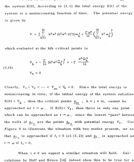
summarized in Figure 1. Under certain circumstances, given in

Section II. 7, part of the solution branch constructed in Section II. 5

is shown to be a branch of minimal positive solutions, in the sense

of Keller and Cohen [19]. Furthermore, conditions are given under

which a branching point is the least upper bound of values >-. for which positive solutions of (1. 2) exist with T fixed. The bifurcation

diagram is completed in Section II. 8, where it is shown that for all values of T sufficiently small, (1. 2) has two distinct solution

branches, although some of these branches may not contain

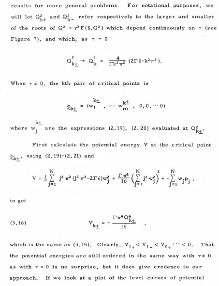
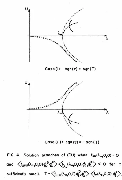
branching points. A graphical summary of the main results in Chapter II is given in Figures 2, 3 and 4.

In Chapters III and IV, these ideas are applied to t1Le dynamic

buckling of arches and imperfect columns and to the buckling of an imperfect column on a nonlinearly elastic foundation, respectively.

In Chapter III, global stability characteristics for the buckled e quilib-rium states of an imperfect column are studied using the qualitative

features of nonisolated solutions discussed in Chapter II. In Chapter IV,

an advantage in using the present iteration technique in problems of imperfection sensitivity in buckling is demonstrated. It is a simple consequence of our approach that an approximate solution of the

buck-ling load is asymptotic to the exact solution. Approximation techniques used elsewhere do not have this feature [3].

Equation number (1. 1) refers to the first equation of Section 1 of the given chapter. Similarly, Theorem 3-1 refers to the first

theorem of Section 3 of the given chapter. When referenc.e is made

Chapter II

General Imperfection Theory

II.l. Notation and Definitions.

We want to study branching phenomena for elliptic boundary

value problems of the form

(1. 1) Lu

+

Bu = 0 x E

aD .

Here x = (x_{1 ,} , x ) and L is the uniformly elliptic second order

n

operator defined on D by

(1. 2)

n

\' 82 _u

Lu

=

i,j=l 1 J

n

\'

au

+

o

x

.

J

- a

(

x

)u .

The boundary operator

B

oD

(1. 3) Bu

=

(

x)u

+

n

b 1 (x)

~

au

ox.

J

where for notational purposes we will denote

n

~~

~

j=l

f3.(x)

au

ax.

k+a

We denote by C (0) the space of real valued functions which are k times continuously differentiable on a point set

n'

0

aD

>

1J J

to be in Cz+a(D) , C1+a(D) and Ca(D) respectively, while b₀ (x) , b₁(x) , f3.(x) are in CI+a(aD) for some aE(O,l).

1 The uniform

ellipticity of L implies that for all unit vectors y = (y1 , ••• , y n)

n

(1. 4)-i)

I:

1J 1 J XED .

i,j=l

Taking n. (x) to be the components of the unit outward normal at 1

X E an, we assume that the coefficients of the boundary operator B

satisfy

n n

(1. 4) -ii)

~

13.

>

I:

J J J

j=l j=l

and that an can be decomposed into an = an1

U

(1.4)-iii)

(1.4)-iv) b0 (x) ~ 0 b1 (x)

>

The assumed smoothness assumptions on L and B are

Q '

-9-(1. 5) Lu(x)

=

xED

Bu(x)

=

xe:aD

2 + a

-has a unique solution, u(x) E C (D) ( [26], pp 134-136). These

assumptions further imply that L and B satisfy the strong maximum

principle [ 31] which leads to

Proposition (1): If cj> (x) E C' (D)

n

i - Lq> ~ on D , B q> ;::,: 0 on

an

ii - Lq>

<

Bq,;::,: 0

an

;:::.

>

0

D

Furthermore, if cp(x)

=

aD,

aq,

aa

<

xe:aD

where

a:

We will assume that the nonlinearity f(A., T, u) satisfies

f(A., 0, 0)

=

a 2+a

assume that f(A., T, u) E C (D) whenever u E C (D), and the partial

derivative at A., T,u satisfies f (A., T, u) E Ca(D) when u E CHa(D). All u

other derivatives up to and including third order are assumed to be

continuous on D if u E C2+a (D). Although f(A., T, u) is allowed to

The standard bifurcation problem with T

=

[21], [25], [34], [38] ).

of these studies

[25]

(X._{0 ,} 0) only if there are nontrivial solutions of the problem

(1. 6) xED

Bcjl = 0 x E

an.

For the forced case with To

*

point of (1. l) only if there are nontrivial solutions to the problem

resulting from linearization of (1. l) about the known solution at X.

=

That is, there must be nontrivial solutions to

(1. 7)

Ll)J

+

=

Bl)J

=

x ED

XEOD

where (X._{0 , To,} u_{0 )} satisfy (1.1). Solutions (u, l)J, X., T) satisfying both (1.1) and (1. 7) will be referred to as non-isolated solutions of (l.l) corresponding to the point X..

To provide a starting point for our investigation, we will

assume that there is a number X.₀ and a nontrivial function

z+a-<Po (x) E C (D) which satisfy (1. 6). The quadruple (u, l)J, X., T)

=

(0, <Po, X._{0 ,} 0) will be referred to as a trivial nonisolated solution of

(l.l). We will also assume that all solutions of (1. 6) are multiples

(1. 10)

By defining the inner product

(u, v) =

J

D

.. ,..

,.,

we can define adjoint operators L~ and B' to be those operators

satisfying

(1. 11) (v, Lu) - (u, L

*

=

z+a-

,:,

whenever u, v, E C (D) and Bu = 0, B v = 0. The operators which

result from this definition are given by ( [

6]

, [13])

n ₈2

(a .. (x)v) n

)!:::

(1. 12) Lv

=

~

ax.

ox.

~

8(a. (x)v)

ax. - a0 (x)v , x E D .

i, j=l 1 J j=l J

B,:,v = 0 is defined by requiring

(1. 13)

n n

P[u, v] =

~

~

L

ux. lJ l

i,j=l 1 J i=O

x E

oD.

when Bu = 0. For p(x)EC (D), a - whenever

(1. 14) L<j:>

+

=

B<j:>

=

has a nontrivial solution, we know from the study of spectral theory

>:~ >!<

··-(1. 15) L <j>

+

=

'~ ~~

B <j>

=

also has a nontrivial solution, and the null space of equation (1.14)

is of the same dimension as the null space of (1.15). The Fredholm Alternative Theorem [6] holds for solutions of

(1. 16) Lv

+

=

Z

+a-Specifically, this asserts that (1.16) has a solution v(x)E C (D)

a -provided g(x) E C (D) and

(1. 17) ( g(x) ,

<Po)

=

where

<j>'~

function11 _{such that}

(<P

o

0(x) A(x) ) of. 0. We make the stronger

assumption that if the solution v(x) in (1. 16) is made unique by

requiring the orthogonality condition

(1. 18)

,.,

( v(x) , <j>~ (x) A(x) )

=

then there exists a constant G> 0 such that

The notation has been chosen with an eye toward general

-izations. If we wanted L to be an operator in a real Hilbert space

H, then the inner product (1.10) could be chosen appropriately. The

inequality (1. 19) could be assumed to hold in the induced norm of

H, and many of the results that follow would be true with only a

slight change of wording.

II. 2. Perturbation Theory for Non-isolated Solutions.

Formal perturbation theory is often used to obtain useful

approximations to solutions of nonlinear boundary value problems.

The ideas used in the method originated in the work of Lindstedt

and Poincare [30] on periodic motion in celestial mechanics.

Recently it has been applied by J. B. Keller and others [22], [23] ,

[29] to a number of nonlinear boundary value problems arising in

such diverse areas as nonlinear optics, heat conduction, and

super-conductivity.

In this section, we will develop a formal perturbation scheme

which indicates the form of nontrivial non-isolated solutions of (1.1).

We will show that this scheme is well defined and can be carried

out to arbitrary order provided the nonlinearity f(:>-., T, u) is sufficiently

differentiable in each of the arguments :>-., T and u. It will be the

task of later sections to show the validity of this perturbation

scherne.

nonis olated solution of (l. l). Our hope is that this solution is an

element of a branch of nonisolated solutions, and that this branch

can be represented parametrically with some parameter E . If

this parametric representation is also sufficiently differentiable at

the known s elution (u, ljJ, A., T) = (0, <Po, A._{0 ,} 0), then we can expand the

parametric representation in a Taylor series about known solution.

We choose the parameter E so that (u(x,E), ljJ(x,E), 'A(E), T(E))

=

(O,<j>₀ ,A.₀ ,0) when E=O.

The first n+l terms of this Taylor expansion will be referred

. to as the nth perturbation expansion for nonisolated solutions of (l.l),

and will be in the form

( 2. l)

...__n

u (x, E) = € (u0 + E u1 + · · · + E u ) n

n

""n

ljJ (x, E) =

n 'A0 + E 'A 1 + · · · + E 'A _n

n

E (To + E T1 + · • · + € T ) .

n

There are two equivalent ways to determine the coefficients

in (2.1). Since (2. l) is intended to be the Taylor series of solutions

of (l. 1), (l. 7) about € = 0, one could differentiate (l. l) and (l. 7) k

times, and then set € = 0, thus finding the equations which

deter-rnine the coefficients of the kth terms as functions of the previously

dete rn1ined cOl' ffic- i0nts. Alternately, one could substitute expression

powers of E , and then equate coefficients of like powers of E . The equations which result will again determine the kth set of coefficients

as functions of previously determined coefficients. Since these two methods are equivalent, both require that the nonlinearity f(}.., T, u) have smooth derivatives of at least order n.

(2. 2)

(2. 3)

(2. 4)

(2. 5)

Carrying out the above expansion procedure, we get

Lu₀

+

=

=

Lu₁

+

u

xEaD

L¢₀

+

xE

a

XED

xE aD

xED xED

*·

Since the operator L

+

~!;:

by <Po , we know by the Fredholm alternative theorem that

equations (2. 2) - (2. 5) can be solved if and only if the right hand >:C

side of each equation is orthogonal to q,₀ as in (1.17). This

con-dition determines the constants >..._{1 ,} To and T₁ in (2. 2) - (2. 5).

Furthermore these solutions will not be unique, since we may add

any multiple of q,₀ to the solution. To make the solutions unique,

we require

>:c

( ljl(x),q,0 (x) fX.u(X.0 ,0,0)) = 1 (2. 6)

*

( u(x), q,₀ (x) fX.u(X._{0 ,} 0, 0) ) = €

This places a restriction on the terms of the perturbation expan-sion (2. 1), requiring that

*

( q,o, q,o fXu (X.o, 0, 0))

=

*

( uo, q,o fX.u(X.o' 0, 0))

=

and

*

(ljl.

,q,

1 u

(2. 8) i = 1, 2,

*

( u., q,₀ fX. (>..._{0 ,} 0, 0) )

=

1 u

In order to solve (2. 2), the Fredholm alternative theorem

requires that

(2. 9) To ( f (>,._{0 ,} 0, 0) , <Po

*

T

*

Assuming that (f (X._{0 ,} 0, 0) , <Po)* 0, we must have To= 0. With

T

To

=

(2.10) _{u 0} (x) = <Po (x) .

Using this information, equation (2. 3) becomes

(2.11) xE D

xE

aD.

Applying the Fredholm alternative theorem to (2.11), we have

(2.12)

Similarly, from equation (2. 5) we get

Equations (2.12) and (2.13) are two linear sin1ultaneous

equations for >--.1 and T 1 . The determinant of this systen1 is

(2. 14)

so that these equations can be solved provided D

*

*

solution of (2.12) - (2.13) is

2 'l<

(fuu(>--o,O,O), <J>o,<J>o)

....

(f>--.u (>--o' 0, 0) <Po'

<j>; )

(2.15)

2 >:.C 1 (fuu (>--o' 0, 0) <Po , <Po )

Tl

=

*

( f ( >--.0 , 0, 0), <Po )

T

Of interest in many applications is the relationship between

>--., the "buckling load," and T, the "imperfection amplitude. 11

According to (2. 1)

so if _{T 1}

*

(2.16)

and

2

*

...._ =

C

2

<J

(>--.0 , 0, 0), <l>o, )

(2.17)

can be combined to give

2

*

(fuu P.-o' 0, 0) <Po' <Po )

*

(fx_u(X.o,O,O)<j>o,<l>o)

(2. 18)

'K

TYz

)'C: 2 , ....

[2(fT(X.

₀

0

0

:~

(fx_u(X.o,O,O)¢o.<l>o)

where T must be restricted so that X. is real.

Yz

+

In many applications, f _uu (X.0 , 0, 0)

=

valid. Suppose there is an integer p such that

(2.19)

k

a

<

auk

=

aP+1f(X.₀ ,0,0) aup+I

2 ~ k~p

p+I ,,,

<Po , ¢o' )

*

Then the perturbation equations can be shown to reduce to

(2. 20)

(2.21

Luk + fu(X.0 , 0, O)uk = 0

Buk

=

Lup

+

= -

+

+

J

Bu = 0

p

T p

x €

aD

xED k=O,l,2, ... ,p-1

x€

aD

aP+ 1 f ( X.o, 0, 0) aup+I

X€ D

and

(2. 22) X€ D k

=

B4\:

=

[

aP+1f('X.₀,0,0)

{

Llj;k+fu('X.0,0,0)lj;p=- 'X.pf'X.u('X.0,0,0)<j>0+ ()up+₁

(2.23)

B·'· _'~"p =0 xE8D '

and the conditions (2. 7) and (2. 8) are required to hold.

According to equations (2. 20) and (2. 21),

(2. 24)

{

u₀ (x)

=

k = 1, 2, ... p-1 ' p+1 <l>o

- ₁ ] ,xED

p.

and the calculations used in deriving (2. 20) - (2. 23) show that

(2.25) k

=

Using (2. 24) and (2. 25) in (2. 1), the form of the solution reduces to

~p

(2. 26)

:;:-P

= E (<Po + Epu ) + O(Ep+Z)

p

=<j>₀ +Eplj; +0(Ep+1)

p

=

0 + Ep'X. +

O(Ep-1-1 ) p

P

+

Invoking the Fredholm alternative theorem in (2. 21) arid (2. 23), we

can find }...p and T p" Specifically,

(2.27)

=

*

=

p

so that

(2. 28) T =

-,-P~-p

1 ap+t f(}...0, 0, 0) p+I

(p+ 1)!

<

1 ap+t £(}...0,0,0)

<

p! _aup+l

*

T

<!>o

p+l

<!>o

*

>

*

>

At the outset, we assumed conditions (2.19) that assured us that

T -=t- 0. Now we can solve for }...

=

we get

(2 .29)

p

p+l

}... :}... _ _ T _ ((p+l)!

0 p! p

Thus, the buckling load }... is altered by imperfections in the order

of Tp/p+ 1 for T sufficiently small.

We would like to show that the perturbation scheme given by

(2. 1) is well defined, and that the kth terms of the expansion are

previously determined k terms. If we assume that f(>-., T, u) is at

least n+2 times continuously differentiable in all variables, then

expanding f(>-., T, u) in a multivariable Taylor series with remainder

near >-. = >-._{0 ,} T = 0, u = 0, and substituting (2.1) into the Taylor

series, it is easy to see that

(2. 30) _+~~(

~

1cr

+ Pk{ u0 , • · :uk_₁;

>-

·,~_

1

;

J

(2. 31)

On substituting (2. 30) and (2. 31) into (1. 1), (1. 7) we get

(2.32)

"'"'n

Bu

=

and { _Llj! ""n _{+fu(>-.0,0,0)lj!} ""n _=-~

f,

[~

l

1

(2.33) J- xED

Equating like powers of E, we have

{

Luk

+

=

~

+

+

(2. 34)

Buk

=

an

=

XED

XED

As before, equations (2. 34) and (2. 35) can be solved only if

the Fredholm alternative is satisfied. Using that u₀ =

lJ.Io

resulting equations are

(2.36)

and

Notice now that using equations (2. 34) - (2. 37) determines the kth

terms of the expansion (2.1), uk, lj.Jk , X.k and Tk as functions of

the previously determined k terms. The equations (2. 34) - (2. 37)

are linear, and involve the same differential operator and matrix

operator for each term of the expansion. This assures us that the

D of (2.14) does not vanish, and provided f(A, T, u) is sufficiently

differentiable. The condition (2. 8) makes the procedure unique.

The solutions of (2. 36) and (2. 37) are

and

k-I

(f (A O

~)

[1::

((f

₀

₀

;T0;··,T._})

0• , , 0 U/\. J J J I J I J l

T .

J:::l

When the coefficients ~ , tVk , Ak and Tk are substituted into (2.1),

the resulting expansion is an asymptotic solution of (l.l) for E

suf-ficiently small. This fact will be shown in Section 4.

II. 3. Existence of Non-isolated Solutions.

In Section II. 2, we were able to develop a perturbation

scheme which gave rise to expressions which we hope are

approxi-n1atc solutions of (l.l), (l. 7). At this stage, however, we do not

even know that (l.l), (l. 7) have "nontrivial" solutions. In order to

in a form suggested by the perturbation m ethod, namely

(3. l)

u(x,E)

=

=

T(E) = EZl'/(E) ,

where

cJ>o

6).

*

(v(x,E) , cj>₀ (x) f>-.u(>-.0,0,0)) = 0 (3. 2)

(x(x,E)

We must show that for some nontrivial range of the parameter E,

0 ~ jEI ~ E₀ , the functions v(x,E), x(x,E), !J.(E), l'/(E) exist and are

bounded uniformly in E . If this can be shown, then as E approaches

zero, the solutions (3.1) approach the trivial solution (u, ljJ, >-., T)

=

(0, cj>_{0 ,} >-._{0 ,} 0) continuously. Furthermore, the solutions (3. l)

cons-titute a family of nonisolated solutions of (1. l) depending continuously

on the parameter E .

To carry out the analysis for this problem, we will make

use of the identity

(3. 3)

1 dg

g(a) - g(b) = (a-b)

J

0

dg

To use this identity for (1.1), (1. 7) we will assume that f(X., T, u)

has at least three continuous derivatives in X., T and u. Substituting

(3.1) into (1.1) and (1. 7) gives

(3 .4)

and

(3.5)

u € u

r

-~-11

J

1

fT(X., s T ,u)ds +

ra-(

<j>

0

+~t

- 0 0 0

2

j

'

lll

J

+ (<j>₀+Ev) f (X.₀ ,0,stu) sdtds

0 0 uu xE D

= P(v, f.J., 11, E ;x)

Bv = 0 , x€ 8 D

LX+ f (X.₀ ,0,0)x=

_1_~-f

4J

u € u u

"'_ff.J.J\

L

0 AU 0 TU

+ (<j>o+Ev)j. 1

f (X.₀,0,su)ds] (<j>₀+EX) 0 uu

=Q(v,x,f.L,11,E; x) xED

Bx

=

o

Equations (3. 4) and (3. 5) are of the form (1. 16) and can be solved for

v and X only if the orthogonality conditions

>:.::

(P(v, f.J.,11,E; x), <Po )

=

(3. 6)

,,.

hold. These solutions, i f they exist, arc only determined to within an additive multiple of

<Po,

The orthogonality condition (3. 6) provides the m ethod by which we intend to solve (3. 4) and (3. 5). We will solve them iteratively, first by choosing values of

n

scheme is a modification of the standard technique of Lyapunov and Schmidt ( 38] suggested by the treatment in

[17)

problem (1. 1) with T

=

To formulate the contraction mapping we introduce the sets of functions

I

-(3.7) BK={y(x) y(x)EC (DJ,!IYII~K ,(y(x),<j>~-(x)f:\u(:\

0

and the real interval

(3. 8)

Notice that

s

r)

pr

r

BK

n'

where

j

*

((<j>o+EX) 0

fX.u(X.₀+ sE fJ., 0, u)ds, <Po)

(3. 10)

=-

f (X.₀ ,0,

su)ds,<j>~)

0 uu

l

-Er]((<j>₀+EX) f (A,ST,U)ds,<j>~),

0 TU

-

-

r- (

L v + £ u (.~0 •

o . o,

= -

c,

0

r

x..

-

rir

+ fJ.(cpo+Ev)J 0J0

~(X.₀+SEfJ.,O,tu)dsdt

(3.12)

+ (¢₀+Evt

JJif

0 0 uu

(3. 13)

Bx

=

aD

-29-1

+En(<j>0 +Ex)J f (J\.,sT,u)ds

0 TU

This definition of T induces an iteration procedure in a E

natural way. Suppose we let an initial iterate be ( v 0 (E, x),

x

f-lo (E),

n°

v (E,x), X (E,x), 1-l (€),

n

{ ( v v v v ) }

( 3 .14) _[Vv+l, Xv+l, _r-11

V+l

n

v+l]

=

[

x .

n

VJ

.

We are now able to state and prove the following

Theorem 3-1: Let S1 = S₁ (p, r) for some fixed p ~ 1, pr ~

1.

Suppose that

(3. 15) and

f (J\. T u) f f f f f f f f . f

T 1 1 1

J\.1

}\u' UU1

TU' uuu' J\.uu' TUU' TTU J\.J\.u

*

and that (f _T (>. .. 0 , 0, 0), <l>o) ( <l>o f}..u 0'-o, 0, 0), <l>o

*

r

into UK , and TE is a contraction on UK for all E 0 ~ IE I~ E 0.

Furthermore, the problem (1.1), (1. 7) has a nontrivial solution of the form (3.1) where v(x,E), X(x,E), j-L(E), 7'}(€) satisfy (3. 4) - (3. 6) and are the limits of the iteration scheme generated by TE for any initial iterates in UK

( 3. 16)

Proof: For notational purposes, define

= sup

I

I

Since S1 depends on the numbers

p

pr

r

r.

p,

pr.

II

II

=

=

By virtue of the smoothness assumptions we made about inverting the operator L

+

U E

maps UK into

'l1<: ,

~

SJK .

*

We assumed that

I

-

31-(3.17)

for _{X.,T,U)ES1. Then if (v,x,f.L,l"J)EUK for some _{E 1 ,K} with E₁~1,

E 1 K ~ 1 , we have

{3. 18) {

I~

~

.f

II

II

J

~ At

+

(3.19)

- 2 [ - z

II

lnl

~13

I~J.I{II<!>II

00

+E1K)IIfux.lls+{ll<t>lloo+E

1

K) ~

2

-~ A₂

+

{3. 20)

and

(3. 21) {

II

X

~

[1

~I

II

II

II

II

II

II

+ E 1 K II f II

J

~

*

where <1?

=

(1,

(3.22) A.

+

1 1 i = l , 2 , 3 , 4 .

This is easily accomplished, since B. (E ₁ ,K) depend continuously on 1

E 1 and K, we can pick K

>

{A.}

,

>

0

i=l,2,3,4 l 1

so that ( 3. 22) holds. Letting Ez=min{l, K, E_1} we have that

TE: UK- UK for 0 ~IE I ~ Ez. The second part of the proof involves finding Eo ~ e2 so that TE is a contraction on UK for 0 ~ /el~ e0 •

Suppose we let w1 = (v,x,!J-,1]) eUK and w2 = (y,z;,,v,K)eUK. Then we

can show that there exists a positive constant M such that

(3. 23)

where

In particular, with some straight forward calculations, it 1s easily shown that

(3. 24)

(3. 26)

and

(3.27)

where

II

~-y

IL

~

IE I [

A~nll

v-y

IL+

11-L-v

I

+ A33

ITJ-K 1]

+

A:34

I~

-K

I +

A:3s

I~-~

I

•

lix-~ II~

IE

I [A4tll v-y II+

A4z

llx-l;, II+

A4311-L-v

I+ A44 ITJ-K 1]

00 00 00

Au=~~=(II<J>I!+l)[ll£

11+11£ .. II+E

(II<J>II+l)ll£

II+Ezllf

II,

A1z = A4z =

II

II +II

II

+ (II <l>

II

+1)

II

II

•

A13=~3=

(ll<l>IIJl)[Ez

ll£uX.'TIIs+~ll£uX.X.IIs]•

A14=~4=

(ll<l>llcJ1)[11fu'TIIs+

€~

ll£u'T'TIIs]'

Az

=

(II

<l>

II

oo

+ 1l11

Ll

uu s

II

+ Ebz

(

Jl

<l>

II

oo

+

II

uuu

II

s

+

i II£ ,

uu

II

l_._

II

II

+

II

II

,

1\.

sj

u/\. s

s

Azz

=

A:3z =

~(II

<l>

IIJl)

II

fuX.X.

11

+

II

lis]

•

Clearly,

imply the existence of a constant

such

that

holds.

By choosing

<

<

1, the

mapping

TE is

a

We have now shown that for

jEI

.:::;

Eo,

and is a contraction. But this is not sufficient to show that the

iteration scheme generated by T converges to a solution of (3. 4)

-€

(3. 6). We know by virtue of the contraction that the sequences

and {fJ.v(€)} converge. By a simple induction we also know that

v v z+a

-v (€, x) , X (€, x) € C (D). This allows us to apply the Compact

-ness Theorem 12.2 of Agmon, Douglis and Nirenberg [1] , which

justifies taking the limit v - oo in (3.14).

Q.E.D.

It is easy to see that a solution of the form (3. l) is

unique. If it were not unique, then there would be two solutions,

say w₁ -:/< w₂ which both satisfy (3. 4) - (3. 6). Thus, both w1 and

w2 are fixed points of the mapping T given by (3.10) - (3.13), so

E

that w1 = w1 and Wz = w2 • Applying (3. 23} we see that

(3. 29)

whenever

I

I .:::;

the solution is unique.

The proof of Theorem 3.1 assured us that nonisolated

solutions of (1. 1) are of the form (3. 1), where v(E, x), X(E, x) , fJ.(E),

and TJ(E) are uniformly bounded by K for

lei

about the quantitative behavior of the solution, we would like to

know more about fJ.(E) and T](E). We know that fJ.(E) and TJ(E) are

is an integer p such that

(3.30)

<

aP+I _f(X.0,0,0) ()up+ I

= 0

.hp+I

'1'0 '

<Po

*

)

*

holds, and assume that all third derivatives of f(X., T, u) exist and are continuous. Then applying the identity (3.3) to (3.10) and (3.11)

we find

and

(3.32)

=

Although (3. 31) and (3. 32) include implicit dependence on !J.(E) and

n(e:)

I!J.(E)i

~

I

I

IE

I

asymptotic form of jJ.(E) and

n(e:)

le:

I -

The system (3. 31) - (3. 32) can be solved for E sufficiently

{3.33) !J.(E)

{3 .34)

n

p-1

= -

p+I )

a

+t

*

( p+ I

<P~

' <Po )

au

p+l

a

<Po

,

au

P- I

=

*

<Po

)

Coupling (3. 33) and (3. 34) with the form of the solution (3. 1), we see that the perturbation solution (2. 26) - {2. 28) is asymptotic to the solution {3.1) as E - 0. In section 4, we will show that this is true for the perturbation scheme with any number of tern1s.

II. 4.

In Section 3 we found a mapping T whose fixed point gave

E

rise to solutions of (1.1), (1. 7) for each

E,

\E\

iterations generated by T were found to converge to the fixed E

point for all initial iterates in UK .

In this section, we will examine the iterations generated by the initial iterate

To estimate the errors of the kth iterate w , k we apply (3. 23) to get

(4. 2)

where _{€ 0} 1s chosen so that _{€ 0} M

<

1.

find that

(4. 3)

{

A simple application of the triangle inequality implies

(4. 4)

=

K(le IMt

<le

IM)m

1-

leI

and passing to the limit as m - oo , we get

(4. 5)

where w

=

We can interpret this information in terms of the solutions

of (1.1), (1. 7) in the form (3.1). The sequence {wk} corresponds

for € fixed to finding a sequence (uk (E, x), lj;k (E ,x), f.Lk (E), TJk (E))

where

k

k

u (E, x) = E <j>₀

+

k k

ljJ (€, x) = <j>₀

+

X

(4. 7)

k

X.0

+

k 2 k

T (E)

=

n

with initial iterate

(4. 8)

Furthermore, (4.6) tells us that

( 4. 9)

We would now like to show that the perturbation method

-39-E - 0. Specifically, we will show that (4. 9) holds for the iterates (4. 7) and also for the perturbation terms (2.1). To do so we

prove the following

Theorem 4-1: Let the hypotheses of Theorem 3-1 hold, and let (2. 30) and (2. 31) be satisfied for all E ,

I

. n n n n

Then the 1terates (u , ljJ , X. , T ) of ( 4. 7) and the perturbation

-n -n -n -n

expansions (u , X. , X. , T ) of (2.1) and (2. 34) - (2. 37) satisfy

11

n -n

u (E , x) - u (€ , x)

II

(4.10)

Note that applying the triangle inequality with (4. 9), (4. 10) assure us that the perturbation method is asymptotic to the known solution

as

E-o.

Proof: The proof of a similar fact for the bifurcation

v+I

X. -X.o. v v v v v

*

*

(4.11) ( ·1(f (X. ,0, u )\jJ -f (X.₀,0,u )\jJ

,cp

0 )

X.v _ X.o u u u u

v+I "' ,v+I , "'

T V V V . V V -.< ( f\. -f\.Q V V V -r-- (f(X. ,T ,u )-f(X: ,O,u

),cp

0,0,u

),cp

Tv ~-X.o

(4.12)

v v ~~

=- (f(X._{0 ,} O,u ) - f (X.₀,0,0)u, ¢>o ) ,

u

[ v+I

v+ I v+ 1 T v v v v v

Lu

+

=-

0(X:,

T

(4.13)

Buv+l

=

v v v v v

+

u u

(4.14)

v

J

+

provided Tv io: 0 and

X

v

T

is replaced by f (X.v,O,uv) in (4.12) and (4.13).

T

Similarly, if X.v = X.₀ , the

expression fu(X.v,O,uv)-fu(X.₀ ,0,uv)/ >...v->..₀ is r eplaced by f>...u(X.₀ ,0,uv)

in (4.11) and (4.14), and f(X.v, O,uv)-f(X.0 , 0, uv)/>...v ->...0 is replaced by

fA(X.₀ ,0,uv) in (4.12) and (4.13).

Suppose that (4.10) holds for some n> 0. This implies

n -n

u = u + E n+z e (E) ,

n

I

I

I)

l)Jn=~n+En+len(E)'

II

(4.15)

n -n

X. =X. +E n+l

1-Ln

11~-Lnll

linn

II

n

Applying (4.15) with (2. 30) and (2. 31) we see that

(4.16)

and

(4.17}

n n n n n n

f(X , T , u ) = f (X.₀,0,0)u + f (X.₀,0,0)T +E f, (X.₀,0,0)u₀(X ->...₀ )

u T ~u

n+l

+

L:

,~-l

;

k=l

n n n n

f (X , T , u )

=

+

u u u~

(4. 18)

n+I

~+I

=

k=O

then (4.17), (4.18) combined with (4.11) give

k=2

n+I k n+I

(4.19) = - I Ek I

(Qj{u

0

,'~uj_

1

;'X.

1

,"','X.j_

1

;

T

0

,'

"

,Tj_

1

}l\ik-j'<j>~)+I

k=l j=l k=2

where

where 'X.k, Tk' uk and

lJic

=

n+I k

n+l, then the polynomial :L E qk vanishes identically, and the k=z

corresponding terms involving this polynomial are n+I k

In

(4.19). If p~n, then .1: E qk :l:E k+E f-Ln is

k:Z k=I

not present in a polynomial of order E • In either of these cases, equating the coefficients of E in (4. 19) gives

Comparing this with (2. 38) we see that !3I = "-I. In fact it is easily

seen that !3k = A.k for k = 1, 2, · · · , min(p, n+l).

If p ~ n we must still determine !3k for k ? p+l. Suppose

that for some k ;t p+l, !3 = A for v

<

v v

(4. 20)

n+I k

:£: € !3k k=I

=

n+I k p+I .

Since 2,; € qk is a polynomial of order E , equahng the

coef-k=z

ficients of ek in (4.19)

k

(4.21) !3k(f '(A.o, 0, 0 )lfio,<P6)

= -

\'

·,x.. ;

u 1\. j~ I J

ri

ri

ri

k-1

j=I

which upon comparison with (2. 38), shows that t3k = Ak. This

process can be carried out for all p+l ~ k ~ n+ l , which completes

the induction necessary to show that

n+I ~

(4.22) An+I = Ao +

~

k=I

In a similar manner, combining (4. 12), (4. 16) with (4. 20} and

k=o

(4.23)

where

k=l

n+1

- E

~

~uk_

1

,o;

·

,o},<J>~)

+E k=1

n+t k ~ E 'Yk k=o

n+1

k=1

where we have assumed Tn+I (E) to be of the form n+t

(4.24) Tn+l = E

~

k=O

The argument is now exactly the same as the argument given above and will not be repeated. The result of the argument is that

fo r k = 0,1, ... n+l, or that

n+l

(4.26) T n+t

=

LJ

+

+

The final step of the inductive argument involves substituting

(4.16), (4.17), (4.22) and (4.26) into (4.13) and (4.14). In light of

(4. 20) and the similar relationship for the quotient Tv+1/Tv , it 1s

easy to see that

( 4. 2 7) X E D '

x E

aD,

and

(4.28) XE D '

XE 8D.

The right hand sides of (4. 27) and (4. 28) consist of the differences

of right hand sides of (4.13) and (2. 32) and of (4.14) and (2. 33)

respectively. Since each right hand side expression is orthogonal

*

to

cp

inverse of the differential operator L

+

u

(4. 29) II u n+I_;;n+I Jl

=

00

and

The expressions (4. 22), (4. 26), (4. 29) and (4. 30) are of the form (4.10), so the induction argument, and hence the proof of the

theorem, is complete. Q.E .D.

II. 5. Extension of Solution Branch from Nonisolated Solution.

In the previous sections, we showed that there are non-trivial nonisolated solutions of (1. 1) depending continuously on a parameter E for

I

cum-stances under which a nonisolated solution of (1.1) is an element of a nontrivial solution branch with T fixed. To do so we will

construct the solution branch of (1.1) which contains a given non-isolated solution. A similar problem has been treated by Dean and Chambre

[8), [ 9).

Suppose To* 0 is fixed arbitrarily. If we make the identification

(5. 1)

equation (1. 1) becomes

(5. 2)

g(X.,u)

=

Lu

+

=

XED ' xE an

nonisolated s elution of (5. 2) for X.

=

*

Accordingly, there exist

functions l!Jo (x) and l!Jo (x) which satisfy

(5. 3)

and

(5. 4)

LljJ

+

BljJ = 0

L* l!J*

+

=

*

BljJ = 0

X

ED

'

xE8D

XED '

x€8D

respectively, where g (fJ.o ,w₀ (x)) is the partial

u derivative of g(A., u)

*

*

at (fJ.o

,

w

We will assume that all solutions of (5. 3) and (5. 4) can be rep

-,.,

resented as multiples of l!Jo (x) and ljJ~ (x) respectively. With these

assumptions, the Fredholm alternative theorem (1.16) - (1.19) is

applicable when solving equations such as (5. 3) with a nonzero

right hand side.

We want to find solution sets (fJ.,w(x)) of (5. 2), if they exist,

such that fJ.-fJ-₀ and w(x) - w₀ (x) are small. A natural way to

pro-ceed is to use the perturbation method to suggest the form of such

solutions, and then to construct a contraction mapping which shows

that the suggested form leads to solutions. Suppose we assume an

~(x,

=

+

+

+

(5. 5)

Substituting (5. 5) into (5. 2), expanding g(;;,

~)

o,

equating the coefficients of like powers of

o,

(5. 6)

(5. 7)

and

Lw₀

+

=

Lwl

+

=

=

XED •

XE

aD

XED •

XE

aD

,

Lwz

+

= - [

+

(5 .8)

+

+t

J

Bw2

=

an,

provided the derivatives gX., gX.X.' gX.u and guu exist and are con-tinuous. In order that w₂ be uniquely determined we require that

(5. 9)

-49-Equation (5. 6) is automatically satisfied by our definition of

JJ.o and w₀ (x). Because

4;

theorem implies that (5. 7) can be solved only if

(5. 9) JJ-1 (g

x. (

*

=

*

If we assume that (gx_(JJ.₀ ,w_{0 ),}

4;

*

(5.10) JJ.I

=

=

4;

Finally, the Fredholm alternative theorem applied to (5. 8) gives us

that

(5. 11)

Thus, the perturbation method indicates that solutions of (5. 2) are

of the form

(5.12)

~(

X

,

+

+

;:;:'(o)

=

+

+

where f.Lz

=

-

z

(guu (flo' wo)lJJo2

'~~

Motivated by the results of the perturbation m ethod (5.12),

w(x, 5)

=

(5.13) fJ.(5)

=

On substituting (5. 13) into (5. 2) we get

(5 .14)

Ly + gu(fJ.o,wo)Y

=

-

~2

=-

[v

f

1

gx.(fJ.o+ 52svlw)ds

0

By= 0

+ (lJ.lo+ 5y)

f

J

1

guu&o.wo+ 5st(lJ.lo+5y)) sdt ds]

0 0

=

XEoD ,

Equation (5. 14) is of the form (1. 16) and can be solved for y only

if the orthogonality condition

(5. 15) <P(y, v, 5;x), ljJ

*

=

holds.

As before, we expect that we shall be able to find a solution

To set up such a procedure we introduce the set of functions

and the real interval

(5. 17)

In addition we introduce the set

For each y(x) in

/3K

JlK

₀

o

o

o

o

by

where

(5.19)

By= 0 , xE

oD ,

(y

Then, after picking some initial iterate (y0 , v0 _{), a sequence of}

iterates { yk, }'} will be generated by

(5. 20) ₍ y k+

1

1)

=

We now state and prove the following

Theorem 5-l: Let S2 =S2(p,r) for some fixed p;:::;l, p r ~ 1. Suppose

that

( 5. 21)

and that

Then

:J

o

that the mapping T

0 given by (5.18), (5.19) maps WM =(BMx_9M)

into W M , and T

-53-Furthermore, the problem (5. 2) has a solution of the form (5.13)

for all

o

o

o

o)

(o)

iterate {yk, vk} generated by (5. 20) for any initial iterate in WM.

Proof: The proof is similar to the proof of Theorem 3-1. We

need to show that the mapping T

0 given by (5.18), (5.19), is a

contraction mapping of WM into W M for appropriate constants

o

and M . Again we will use the norm

(5. 22) sup \ g(w)

I

wES

Because of the smoothness assumptions we have placed on g(A..,u),

to show th<3.t T

0 maps W M into WM we need only find the constants

M and

o

BM

, __9

M.

Since we assumed that \ (g;x.._ (fl-o, w₀ ),

ljJ~

l

=

restrict

o

(5.23)

Suppose that (y, v) E WM for some M,

o

(5. 24)

and

(5. 25)

where

~

=

*

I>

The positive numbers A₁ and A2 do not depend on M or

o,

the numbers B I (M, o) and Bz (M, o) are bounded on compact sets of

(M, o). We can easily find (M, 61 ) so that

(5. 26) i

=

by picking M > max{A1,A2 } , and then finding the largest 61 for

which (5. 26) holds. By picking 62 =min {1,

~

o

T 8 : wM- WM for 0

~

10

~

To show that T

0 is a contraction for I 6 I ~ 60 , assume that

w₁ = (y, v) and w2 = (z, fJ.) are in WM. Then for lol ~ 62 we have

(5. 27)

and

(5. 28)

where

(5. 29)

z

II

{

Au=Azt=(llljJII+l)llg

II

8

+llg,

II ,

00 UU S 00 1\.U S

Clearly, (5. 27) - (5. 29) implies the existence of a constant C

>

that

(5.30)

where wEWM.

Now, by choosing 0

<

<

6 is a contraction on WM

for O~lol~ 80 , where 80 =min(o2,63 ).

To complete the proof we need only observe that the

compact-ness Theorem of Agmon, Douglis and Nirenberg

[1]

did in the proof of Theorem 3-1, and justifies taking the limit as

k - oo in (5. 20). Q.E.D.

The solution given by (5.13) is unique in the sense that there

1s only one solution of that form in S ₂ (E 0,M). If there were two

solutions wi:/=w2 , each would be fixed points of T

0, and (5.30)

implies that

(5. 31)

ll

II

~

I

II

II .

For

I

We could compare the iteration procedure (5. 20) with the

perturbation scheme (5.12). Once again we would find that the

perturbation scheme is asymptotic to the iteration scheme, and that

than carrying out the details of such a proof, we will examine the

asymptotic expansion of the solution (y(o, x), v(o)), which are fixed

points of (5.18), (5.19).

Examining (5. 18), it is easy to see that

(5.32) v(o)

=

z

*

- (guu (!J.o 'Wo) lJ.Io , lJ.Io )

*

2 (g X. ( IJ.o ' w o ) , lJ.Io )

+

Substituting (5. 32) into (5.13) we see that to the order which we have

taken the solution, the exact solution (5.13) and the perturbation

solution (5.12) agree asymptotically as &-0.

Knowing the form of the solution (5.13) gives us information

about those parameter values fJ. for which solutions of (5. 2) exist.

Since fJ.

=

neighborhood of (w_{0 ,} t.J.o) for which tJ.

>

solutions of (5. 2) exist in the neighborhood of (w_{0 ,} f-Lo) for which

fJ. < f-Lo. In either case, the point tJ.

=

the number of s elutions of (1. 1) changes from zero to two or from

two to zero as tJ. changes from tJ. <f-Lo to tJ.

>

cases v(O)

>

*

when (gx_ (t.J.o, w0 ), lJ.Io)

>

Figure l gives plots of t.J.(o) versus &

We have now shown circumstances under which a nonisolated

s elution of (1. 1} is an element of a solution branch of (1. 1) for T fixed.

Since in Section 3 we were able to show that nontrivial nonisolated

solutions of (l. 1) do exist, it is natural to ask how Theorem 5-l

If Eo found in Section 3 is sufficiently small, then the resulting eigenvalue X. = X.0

+

The hypotheses of Theorem 3-1 are sufficient to insure that the hypotheses of Theorem 5-l hold in S1 =Sdp, r) for certain nonzero

p,r,

0

sub-stitute into (5.13) for w₀ (x), l\Jo (x) and f.lo, the nonisolated solutions of (1.1) found in Theorem 3-1 and given in the form (3.1). The resulting solutions of (1. 1) are

u = (E+ 6)<j>₀ (x)

+

+

(5.33)

T

=

where E is fixed, IE I ~Eo .

The solution of (1.1) given by (5. 33) is valid only if lol

<

However, the number 6₀ is not independent of the number E . Notice in the proof of Theorem 5-l that 60 was chosen (cf. (5. 30))

so that

(5.34)

where

1 "

Since (p