Research on the Solar Shadow Positioning Problem

2016 International Conference on Computational Modeling, Simulation and Applied Mathematics (CMSAM 2016) ISBN: 978-1-60595-385-4

Research on the Solar Shadow Positioning Problem

Man JIANG

, Zi-yong WU

and Wen-shuo ZHOU

1

School of Resources and Civil Engineering, Shandong University of Science and Technology, DaiZong Street, No. 223, Tai’an , 271000, PRC

2

School of Electrical Engineering, Shandong University of Science and Technology, Dai Zong Street, No. 223, Tai’an, 271000, PRC

*Corresponding author

Keywords: Solar shadow positioning, Solar elevation, Stephenson accelerate iterative method.

Abstract. This paper is mainly about using the length changes of the shadows to determine the location while the length of the object is unknown. Using the solar elevation as a bridge, we build function models between solar declination, geographic latitude of the observing place, hour angle and the length of shadow, and then use Stephenson accelerate iterative method to help solve latitude positioning model, finally realize the shadow positioning.

Explore the Rule of Shadows’ Length Changes

The length changing of shadows is affected by solar elevation and the height of the object. Solar elevation is related to solar declination, geographic latitude of the observing place and hour angle, so we can make a function model to analysis the changing rules of the length of shadow associated to all the parameters, and then use the rule to determine the position of the shadow.

Assuming that the object is a fixed straight-bar, and according to the literature[1] , we know that the solar elevation h is the angle between the straight line where the shadow is and the line which connect the shadow vertex and straight-bar vertex. Its formula is:

sin h= sinφsinδ+ cosφcosδcos t (1) Among them, represent geographic latitude of the observing place, represent solar declination, represent hour angle. Then we set the length of shadow as , the height of straight-bar as , on the basis of trigonometric function, we can get :

s= l

tan h (2) Through above analysis, s is associate with the height of straight-bar l, geographic latitude of the observing place φ, solar declination δ and hour angle t, so we use Jinshan District in Shanghai as an example to analysis what the relation is between the length and the factors.

(1) The relationship between the height of straight-bar l and the length of shadow s Geographic latitude of the observing place φ is 30°54′00″N; solar declination δ=4.7670°; hour angle t =0(we take time as 12:00); the height of straight-bar l∈[0.5,5]; we can get:

sin h = 0.514 × 0.083 + 0.858 × 0.997 _s= l tan h

(3)

Use MATLAB to draw the relationship between s and l, as it shows in the Figure1.

(2) The relationship between length of shadow s and geographic latitude of the observing place φ

sin h= 0.083sinφ+0.997 cosφ

s= 2

tan h

(4)

Use MATLAB to make the relationship between s and φ, as it shows in the Figure2. (3)The relationship between length of shadow s and solar declination δ [2].

The height of straight-bar l=2m; geographic latitude of the observing place φ is 30°54′00″N; hour angle t=0(Beijing time 12:00); solar declination δ[-23°27′, 23°27′]; we can get:

_s=sin h= 0.514sin2 δ+0.858 cosδ tan h

(5)

Use MATLAB to make the relationship between s and δ, as it shows in Figure3. (4)The relationship between length of shadow s and hour angle t [3]

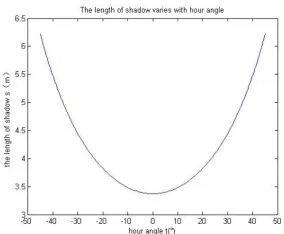
The height of straight-bar l=2m; geographic latitude of the observing place φ is 30°54′00″N; solar declination δ=4.7670°; hour angle t∈[-45°, 45°]; we can get:

sin h=0.514_s= l ×0.083+0.858×0.997 cos t tan h

(6)

Use MATLAB to make the relationship between s and t, as it shows in Figure 4.

Figure 1. The length of shadow varies with the height of straight-bar.

Figure 2. The length of shadow varies with latitude.

Figure 3. The length of shadow varies with solar elevation angle.

Figure 4. The length of shadow varies with hour angle.

Use the Rule of Shadow Changes to Determine the Location of the Observing Place

On the basis of the data of length of shadow of a fixed straight-bar(the bar’s height is unknown), we build a mathematical model to determine the position.

To Determine the Longitude

According to geographic knowledge, when the length of shadow is the shortest , the local time is 12:00, and there is about one hour different local time for every 15 degrees of longitude. The central longitude of UTC/GMT+08:00 is 120°E. we set the time of UTC/GMT+08:00 (It is Beijing time)as t_m , ∆t_m=12-t_mwhen the length of shadow is the shortest; we set the difference between local time and Beijing time as ∆tm, ∆tm=12-tm ; we set the local center longitude is P.

So, the longitude positioning model is:

P=120°+∆tm×15°

∆t_m=12-t_m (7) and

if if ∆∆ttmm=0, the region is located in 120°E >0, the region is located in the east of 120°E

if ∆tm<0, the region is located in the west of 120°E

(8)

To Determine the Latitude

For the determination of latitude, we establish nonlinear equations and use Stephenson accelerate iterative method to solve, finally we use MATLAB to plot to test the result.

At first, we know that the three factor latitude φ, solar declination δ, hour angle t are the three dependent variables of solar elevation angle according to formula (1), then we can work out solar declination δ, hour angle t according to the data and time that we measure length of shadow. We set solar elevation angle h₁(φ) is the function of Moment 1 in a location, solar elevation angle h₂(φ) is the function of Moment 2.

So, the latitude positioning model is:

!

"h1(φ)= sin-1(sinφsinδ+ cosφcosδcos t1 ) h2(φ)= sin-1(sinφsinδ+ cosφcosδcos t2)

tan h₁(φ)

tan h2(φ)

= l s₁ # l s2 # = s₂ s1 (9)

Among them, s₁ is the length of shadow at Moment 1, s₂ is the length of shadow at Moment 2.

The Application of Longitude and Latitude Positioning Model

The Application of Longitude Positioning Model

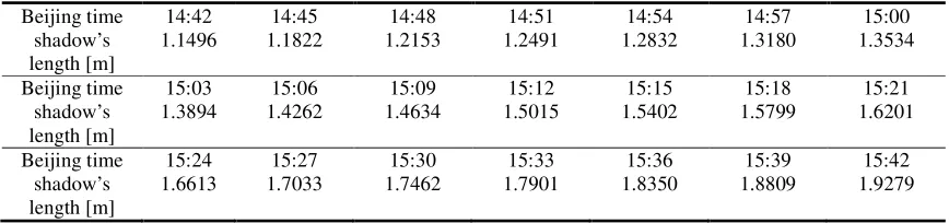
The shadow’s length data of a fixed straight-bar in a certain place are as Table 1.

Table 1. The shadow’s length data at different moments in a certain place.

Beijing time 14:42 14:45 14:48 14:51 14:54 14:57 15:00

shadow’s length [m]

1.1496 1.1822 1.2153 1.2491 1.2832 1.3180 1.3534

Beijing time 15:03 15:06 15:09 15:12 15:15 15:18 15:21

shadow’s length [m]

1.3894 1.4262 1.4634 1.5015 1.5402 1.5799 1.6201

Beijing time 15:24 15:27 15:30 15:33 15:36 15:39 15:42

shadow’s length [m]

1.6613 1.7033 1.7462 1.7901 1.8350 1.8809 1.9279

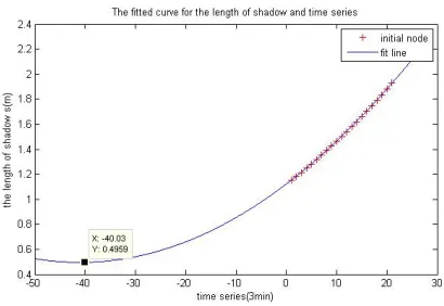
It might be impossible to get the moment (Beijing time) while the shadow’s length is shortest from Table 1 directly. However, we can fit out the function that shadow’s length (y) change with time (x) by using the data of Table 1, and then the moment while the shadow’s length is shortest would be obtained. The function is as follows:

y=3.7226 10−4

× _x2_{+0.0305x+1.1203} (10)

The Figure 2-1 shows the curve of function, in which the lowest point of the curve is (-41.03, 0.4956), which is also the moment point while the shadow’s length is shortest. Now we use t_m to represent the moment while the shadow’s length is shortest, the calculation of t_m is 12:41.

Though the longitude positioning model, we get:P=110°E . So the longitude of the site is 110°E.

Figure 5. The fitted curve for the length of shadow and time series.

Attention: in Figure5, x coordinates each unit length on behalf of 3 minutes. The known data starts from the point (1,1.1496), which represents the shadow length at 14:42( Beijing time). And the lowest point (-41.03,0.4956)represents the moment while the shadow length is shortest, which is 12:41(Beijing time).We can see that the curve fitting effect is very good, so the result moment we get from the function is more accurate.

The Application of Latitude Positioning Model

From Table 1, the measuring date was s April 4th, 2015. According to the date, we can calculate the declination:δ=0.1819rad. We use 14:42 as the start time (represented by t₁ ), use 15:42 as the end time (represented by t₂ ) . t₁ , t₂ are integer degree. At the moment while the shadow length is shortest (t_m=12:41): t=0. So t₁ =30°, t₂ =45°.And we know the shadow length at the two moments: s₁=1.1496,s₂=1.9279.

Then substitute the above data into latitude positioning model, and use MATLAB to solve the system of equations. Write the following code in the MATLAB command window:

Clear all;x0=0.5;tol=0.5*1e-4; [x, time]= Stephenson (‘tan(asin(0.1809*sin(x)+0.8517*cos(x)))-1.667*tan(asin(0.1809*sin(x)+0.6945*cos(x))), x0,tol);

Through changing the initial value x0 ( x0∈(-π/2,π/2) ) constantly, we get three value x ,

x₁=-0.0347rad, x₂=0.3486rad, the number of iterations is greater than 3; The number of iterations is greater than 3; x₃=-1.1921rad , the number of iterations is greater than 2. The margin of error of

the three value x are less than 1.0×10-5. Convert to latitude: x₁=1.988 °S, x₂=19.974 °N , x3=68.560°S.

The Inspection of the Latitude Positioning Model

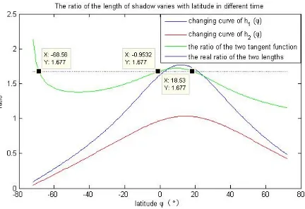
Write the MATLAB program and draw the change curve, then we get Figure 6.

Figure 6. The ratio of the length of shadow varies with latitude in different time.

From the function image, we can see that the latitude φ might be 18.53°N, 0.3803°S, 68.560°S.When compare the latitude result solved by Stephenson accelerated iteration method with the latitude intersections obtained by the function image, we can found that the differences between the two results are small, which also prove the model is reasonable. So we can draw the conclusion that the possible sites are (19.974 °N,110°E ), (1.988 °S, 110°E) , (68.560°S,110°E). In the ideal situation, there should be two latitudes being symmetrical around the declination. However, the earth is not a rule sphere but an irregular sphere whose poles are slightly flattened and the equator is bulging. Therefore, 19.974°N and 1.988°S are not strictly symmetrical around the declination 10°.

Acknowledgments

This work was supported by applied mathematics scientific research innovation team of Shandong University of science and technology.

References

[1] Good search Baike, The Solar Altitude, http://baike.haosou.com/doc/4128005-4327467.html, 2015.9.11.

[2] Good search Baike, Declination, http://baike.haosou.com/doc/4086001-4284778.html, 2015.9.11.

[3] Good search Baike, Hour Angle, http://baike.haosou.com/doc/6834673-7051893.html, 2015.9.11.