Research Article Seabed Identification and Characterization Using Sonar

(1)

Research Article

Seabed Identification and Characterization Using Sonar

Henry M. Manik

Department of Marine Science and Technology, Faculty of Fisheries and Marine Sciences, Bogor Agricultural University, Kampus IPB, Darmaga, Bogor 16880, Indonesia

Correspondence should be addressed to Henry M. Manik,[email protected] Received 5 May 2012; Accepted 27 August 2012

Academic Editor: Joseph CS Lai

Copyright © 2012 Henry M. Manik. This is an open access article distributed under the Creative Commons Attribution License, which permits unrestricted use, distribution, and reproduction in any medium, provided the original work is properly cited. Application of sonar technologies to bottom acoustics study has made significant advances over recent decades. The sonar systems evolved from the simple analog single-beam and single-frequency systems to more sophisticated digital ones. In this paper, a quantified sonar system was applied to detect and quantify the bottom echoes. The increasing of mean diameter is accompanied by a higher backscattering strength. From this study, identification and characterization using sonar is possible.

1. Introduction

Sonar technologies are most eﬀective and useful for sea-bottom exploration. They are based mainly on the measure-ment, process, analysis, and interpretation of the characteris-tics of signal reflected or scattered by the sea bottom. Sonar is also increasingly regarded as the remote-sensing tool that will provide the basis for identification, classifying, and mapping ocean resources.

There are extensive literatures on the acoustic scattering from the sea bottom [1, 2]. The focus has been on low-frequency features in application such as subbottom clas-sification [3]. Another feature of the sea-bottom scattering has been experimentally observed at a high frequency where the transmitter and receiver are not colocated [4]. This method received contributions both from the bottom surface and subbottom echoes. Most of the data were at grazing angles between 5◦and 60◦, but some data were collected for the interval between 1◦ and normal incidence (90◦). They obtained results similar to those of Urick [1].

One of the acoustic methods to obtain bottom scattering is to use a quantified sonar system (QSS). The QSS can measure echoes generated by reflection and scattering of sounding pulses from the bottom. The observed echo is primarily due to scattering from the water-bottom interface.

2. Method

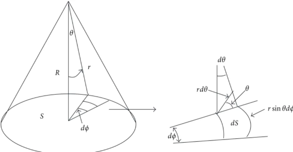
2.1. Sonar Equation for Bottom Scattering. The bottom pro-jection is illustrated inFigure 1. The elemental backscattered power registered by the transducer is given by

dP2

RB=P02r−4exp(−4αr)D4SSdS, (1)

wheredPRBis elemental backscattered pressure signal from

a sea bottom, P0 is source pressure level, r is range, α is

absorption coeﬃcient, D is directivity functions, and SS

is bottom scattering. The elemental area dS is located at incidence angleθ, azimuthal angleΨ, and ranger, such that

dS=r2_tan_{θ dθ dφ.} ₍₂₎

The echo pressure amplitude of sea bottom is obtained by integration of (1):

P2

RB=P0r−2exp(−4αr)ΦSS, (3)

whereΦis equivalent beam angle for surface scattering

Φ= _2π 0 _θ2 θ1 D 4_tan θ dθ dφ. (4)

(2)

θ R r S dφ dφ dS rdθ dθ θ rsinθdφ

Figure 1: Principle of bottom surface scattering.

Sea bottom Bottom echo computation Pre amplifier TVG amplifier SS_SV ERB R

Figure 2: Simplified block diagram of quantified sonar system (QSS).

Figure 3: Quantified sonar system.

The length of pulse in sea water is cτ, and its leading and trailing edges make anglesθ1andθ2as presented inTable 1.

The signal is amplified to give

ERB=PRBMGR, (5)

where ERB is echo amplitude at preamplifier output (V),

M is receiving sensitivity of transducer (V/μPa), and GR

is preamplifier gain (numeric). Combining (3) and (5) we obtain

E2

RB=KTR2 r−2exp(−4αr)ΦSS, (6)

Table 1: Integration limitsθ1andθ2for two cases.

Scattering plane θ1 θ2 Circular plane (R≤r < R+cτ/2) 0 cos −1₌R r Circular ring (r≥R+cτ/2) cos −1₌ R t−cτ/2 cos−1₌R r

where KTR = PoMGR. KTR is transmitting and receiving

factor and therefore

SS= E 2 RB K2 TRr−2exp(−4αr)Φ . (7)

In decibel unitSS = 10 logSS. Simplified block diagram of

QSS is shown inFigure 2.

2.2. Quantified Sonar System. Quantified sonar system used in this research was PCFF80 model manufacturer by CruzPro, Ltd. (Figure 3). The PCFF80 is a full-featured dual frequency (50 and 200 kHz), high-resolution personal-computer-based color fish finder that runs under windows 98, NT, 2000, XP, Vista and Win7 in both analog and DSP mode (digital signal processing). Communications Interface

(3)

106.568656 106.582144 106.595632 106.609120 106.622608 − 5 . 751520 − 5 . 743360 − 5 . 735200 − 5 . 727040 − − 5 . 751520 − 5 . 743360 − 5 . 735200 − 5 . 727040 −

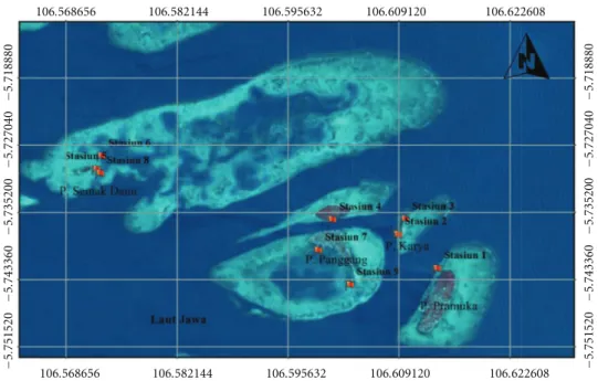
Figure 4: Research location and bottom sampling point.

between transducer and PC was conducted using RS-232 serial data.

For data acquisition, QSS installed on the research vessel. Echo voltages were recorded on hard disc drive. The QSS was operated at a ping rate of about 40 per minute with a pulse duration of 0.4 ms and beam width of 8.5◦.

Calibration of QSS is a fundamental component for ensuring high-quality acoustical data. For this purpose, the acoustic system was calibrated with a 38.1 mm diameter of tungsten carbide sphere. The sphere was suspended under the boat at 0.5 m depth to obtain the transmitting and receiving factor (KTR). The target strength of the sphere at the

given frequencies were calculated following Miyanohanna et al. [5] and Aoyama et al. [6].

By definition, the target strength is given by the ratio between reflected sound intensity,Io, from a target and the

sound intensity transmitted towards the target,Ii, referred

to 1 m distance. This is regarded as identical to the ratio between the backscattering cross section, σ, for the target and the surface of a sphere with a 1 m radius [7]. The target strength can be expressed on a decibel form in the following way: TS=10 log Io Ii =10 log σ 4π (dB). (8)

For simplicity, target strength of sphere was computed using

TS=10 log a2 4 (dB), (9)

whereais radius of sphere.

The equivalent beam angle Ψis the solid angle which is measured in steradian at the apex of ideal conical beam

Figure 5: Collection of sediment sample.

which produce same echo integral.Ψis defined mathemati-cally as Ψ= _π 0 _2π φ=0b 4_θ_,_φ_sin(_θ₎_{dθ dφ.} ₍₁₀₎

In logarithmic unit, equivalent beam angle defined as EBA= 10 log(Ψ) which is expressed in dB relative to 1 steradian.

The specifications of the QSS and calibration results are presented inTable 2.

2.3. Survey Area. An acoustic survey was conducted in conjunction with oceanographic, fisheries biology, and exploratory fishing in the Seribu Island, North Jakarta Indonesia (Figure 4).

2.4. Bottom Sample Collection. Collection of bottom samples was accomplished with a system consisting of a sediment sampler (Figure 5). The bottom sampler was lowered to the

(4)

(a) (b)

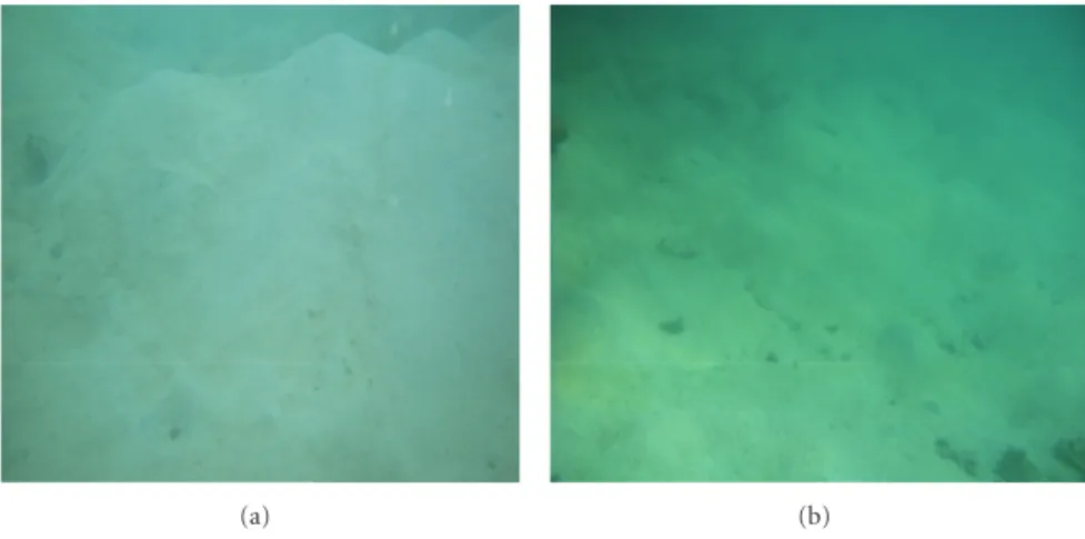
Figure 6: Underwater photography of sand (a) and clay (b).

bottom surfaces by using a diver and entrapped the sediment. The total time of operation for one collection was about 30 minutes.

Bottom samples were separated into size component using sieve separation and pipette settling procedures. Bottom material characterization was based on analysis of particles size distributions conducted during the research.

3. Experimental Results

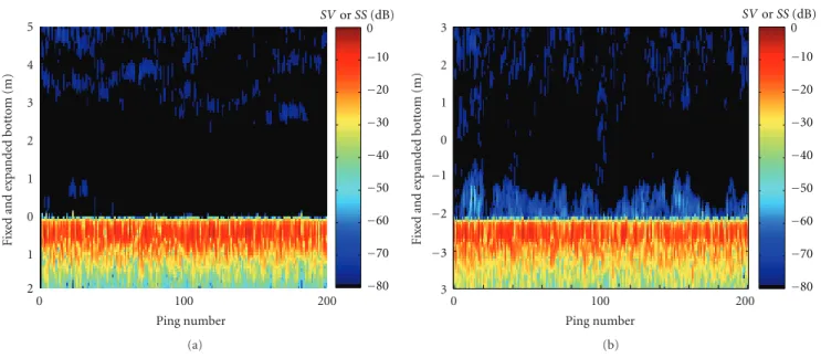
The bottom materials of sand, silt, and clay were determined using observed physical characteristics of the samples and mean diameter were calculated (Table 3). Bottom images from sand and clay and echogram for each bottom type were presented in Figures 6 and 7. Figure 8 shows the bottom backscattering value for three bottom types.Figure 9shows the example echo for sand bottom.

4. Discussion

The quantified sonar system is useful to measure bot-tom backscattering (SS). We had derived bottom volume backscattering strength (SV) fromSSbottom. In this study area, the increasing of mean diameter is accompanied by a higher backscattering strength. The SSof sand is higher than silt and clay by more than 10 dB. To some extent, it was possible to relate SS to mean diameter suggesting the possibility of bottom-type classification and character-ization. Character of the seabed (sediment type, grain-size distribution, porosity, sediment density, sediment velocity, roughness, etc.) are embedded in the sonar echoes from the seabed.

The main reason for the higher backscattering strength with larger particle size is that the porosity of sand sedi-ment decreases as the grain size increases. As the porosity decreases, the density increases (less pore water, more mineral constituent). As the density increases, the sediment impedance increases, thus allowing more scattering from a higher impedance contrast between the overlying water and

Table 2: Specification of QSS and calibration data.

Parameters Quantity

Frequency (kHz) 200

Beam width (deg) 8.5

Equivalent beam angle (dB re 1 sr) −19.0

Band width (kHz) 4

Pulse duration (ms) 0.4

Target strength of standard sphere (dB) −39.1

Absorption coeﬃcient (dB/km) 45.5

Transmitting and receiving factor (dB) 50.5

Table 3: Classification of bottom type by particle diameter.

Bottom type

Sample point

Mean

diameter Sand (%) Silt (%) Clay (%) Sand 1 289 95 2 3 2 305 96 3 1 3 292 94 3 3 Silt 4 45 7 90 3 5 52 4 92 4 6 49 3 93 4 Clay 7 10 3 90 7 8 9 5 91 4 9 11 4 90 6

the sediment. Physically, silt and clay have a higher porosity than sand. Acoustic-bottom interaction is too complex to describe by only frequency and mean diameter. The bottom relief also determines the acoustic echo from the seabed. Because sound may penetrate into the sediments and the subbottom, the echoes can also contain information about the zone below the water-sediment interface. Increasingly, sonar technologies are being used in the future to detect, identify, characterize, and classify the sea bottom.

(5)

100 200 3 2 1 0 1 Ping number Fix ed and e xpanded bott om (m) 0 −80 −70 −60 −50 −40 −30 2 (a) 1 0 3 100 200 Ping number Fix ed and e xpanded bott om (m) 0 −80 −70 −60 −50 −40 −30 −1 −2 −3 (b)

Figure 7: Echogram of sand (a), and clay (b).

−10 −20 −30 −40 0 10 20 30 40 50 Ping number Sand Silt Clay SS (dB)

Figure 8: Bottom backscattering of sand (), silt (), and clay ().

0 20 0 2 4 6 8 10 12 Bottom backscattering (dB) Depth (m) −120 −100 −80 −60 −40 −20 First echo Second echo Sea bottom SS SV

Figure 9: Sand-bottom echo for one ping transmission.

Acknowledgments

The author would like to thank the Directorate General of Higher Education Ministry of Education and Culture Indonesia and Bogor Agricultural University for the Gradu-ate Research Grant Program. Research members are thanked for field data acquisition. He would like to express his very great appreciation to the reviewer for his valuable and constructive suggestions to this paper.

References

[1] R. J. Urick, Principles of Underwater Sound for Engineers, McGraw-Hill, 1967.

[2] H. Medwin and C. S. Clay, Fundamentals of Acoustical

Oceanog-raphy, San Diego, Calif, USA, 1998.

[3] P. C. Hines and G. J. Heald, Seabed Classification Using Normal

Incidence Backscatter Measurement in the 1–10 kHz Frequency Band, DREA, Ottawa, Canada, 2001.

[4] K. L. Williams and D. R. Jackson, “Bistatic bottom scattering: model, experiments, and model/data comparison,” Journal of

the Acoustical Society of America, vol. 103, no. 1, pp. 169–181,

1998.

[5] Y. Miyanohanna, K. Ishii, and M. Furusawa, “Spheres to calibrate echo sounders at any frequency,” Nippon Suisan

Gakkaishi, vol. 59, pp. 933–942, 1993.

[6] C. Aoyama, E. Hamada, and M. Furusawa, “Total performance check of quantitative echo sounders by using echoes from sea bottom,” Nippon Suisan Gakkaishi, vol. 65, no. 1, pp. 78–85, 1999.

[7] E. J. Simmonds and N. D. MacLennan, Fisheries Acoustics:

(6)

International Journal of

Aerospace

Engineering

Hindawi Publishing Corporation

http://www.hindawi.com Volume 2010

Robotics

Journal of

http://www.hindawi.com Volume 2014 Active and Passive Electronic Components

Control Science and Engineering Journal of

Hindawi Publishing Corporation

http://www.hindawi.com Volume 2014

Machinery

Hindawi Publishing Corporation http://www.hindawi.com

Journal of

Engineering

Volume 2014

Submit your manuscripts at

http://www.hindawi.com

VLSI Design

Hindawi Publishing Corporation

http://www.hindawi.com Volume 2014

Shock and Vibration

Civil Engineering

Advances in

Acoustics and VibrationAdvances in

Electrical and Computer Engineering

Journal of

Advances in OptoElectronics

Hindawi Publishing Corporation

http://www.hindawi.com Volume 2014

The Scientific

World Journal

Sensors

Journal of

Modelling & Simulation in Engineering

Chemical Engineering

International Journal of Antennas and

Propagation International Journal of

http://www.hindawi.com Volume 2014 Navigation and Observation International Journal of

Distributed

Sensor Networks

International Journal of