A Meta CSP Model for Optimal Planning

University of Huddersfield Repository

Gregory, Peter, Long, Derek and Fox, Maria

A Meta­CSP Model for Optimal Planning

Original Citation

Gregory, Peter, Long, Derek and Fox, Maria (2007) A Meta­CSP Model for Optimal Planning. In: 

Abstraction, Reformulation, and Approximation, 7th International Symposium, SARA 2007. 

Lecture Notes in Computer Science, 4612 . Springer Berlin Heidelberg, Berlin, Heidelberg, pp. 200­

214. ISBN 978­3­540­73579­3 

This version is available at http://eprints.hud.ac.uk/id/eprint/12217/

The University Repository is a digital collection of the research output of the

University, available on Open Access. Copyright and Moral Rights for the items

on this site are retained by the individual author and/or other copyright owners.

Users may access full items free of charge; copies of full text items generally

can be reproduced, displayed or performed and given to third parties in any

format or medium for personal research or study, educational or not­for­profit

purposes without prior permission or charge, provided:

•

The authors, title and full bibliographic details is credited in any copy;

•

A hyperlink and/or URL is included for the original metadata page; and

•

The content is not changed in any way.

For more information, including our policy and submission procedure, please

contact the Repository Team at: [email protected].

A Meta- CSP Model for Optimal Planning

Peter Gregory, Derek Long, and Maria Fox

University of Strathclyde Glasgow, UK

{firstname.lastname}@cis.strath.ac.uk

Abstract. One approach to optimal planning is to first start with a sub- optimal solution as a seed plan, and then iteratively search for shorter plans. This approach inevitably leads to an increase in the size of the model to be solved. We introduce a reformulation of the planning problem in which the problem is described as a meta- CSP, which controls the search of an underlying SAT solver. Our results show that this approach solves a greater number of problems than both Maxplan and Blackbox, and our analysis discusses the advantages and disadvantages of searching in the backwards direction.

1

Introduction

Optimal AI planning is a PSPACE- complete problem in general. For many prob-lems studied in the planning literature, the plan optimisation problem has actually been shown to be NP- hard [1, 2], whilst the plan existence problem is sometimes only poly-nomial time. For many years, optimal planning has really referred to Graphplan [3] based planners. Successful optimal planners since Graphplan, have relied on its plan-ning graph structure. Notable examples that have also relied on its search strategy are IPP and STAN [4, 5]. SAT based planners, including Blackbox [6], have relied on the planning graph structure, but not the original Graphplan search strategy. These planners convert the planning graph into a SAT model and then allow a SAT solver to search the equivalent SAT instance. One part of the Graphplan search was always kept with these planners, and that was the direction of search. Graphplan constructs the planning graph forwards, until all goals appear non- mutex. It then tests if a solution exists, and if not, then it extends the planning graph by a layer and checks again. This process is repeated until the first satisfiable, and optimal, layer is reached.

Namely, learnt clauses can be shared between layers, if they are still in the context of the previous layer when a satisfying assignment is found.

A problem with this approach is that often finding plans at suboptimal lengths means building redundancy into plans. However, discovering these redundant paths in plans is just as hard as finding a path that actually achieves something. If a goal is achieved early in a plan, there is nothing to prevent the SAT solver from reversing its choice and then later re- achieving the same goal. Especially because the SAT solver has no way of

distinguishing real actions andnoops(actions that maintain a fact’s truth between two

timesteps). This leads to redundant search, and leads the SAT solver to explore areas of the search space that are not interesting in terms of solving the problem. We introduce a Meta- CSP reformulation of the planning problem in which the variables represent the final achievers of goals. The values in those variables represent the actual possi-ble final achievers of the goals, as the SAT variapossi-bles that represent them. We compare the performance of this model with Maxplan and Blackbox. Maxplan provides the best comparison for the meta- CSP model as it uses a traditional SAT encoding with a back-wards direction of search, so any performance difference can be directly attributed to the model. The comparison with Blackbox is slightly less straightforward as the direc-tion of search is different. It will provide some comparison between the two direcdirec-tions of search and provide arguments for when each is more effective.

In Section 2 we introduce the planning problem, the planning graph, and the trans-lation of the planning graph into a SAT formutrans-lation. The meta- CSP model is described in detail in Section 3, comparing it Maxplan and Blackbox in detail. Section 4 and Section 5 show and analyse extensive empirical results from three different problem domains. Section 6 discusses related work and how performance of the model could be improved in the future.

2

Background

Planning is one of the fundamental problems in Artificial Intelligence. The ability to plan and to reason causally and temporally is one of the key features of intelligent behaviour. The planning problem can be defined in the following way:

Definition 1. A STRIPS planning problem P = (O,I,G) has three parts: a set of operatorsO, a set of conjoined factsI that represent the initial state and another set of conjoined factsGthat represent (a partial coverage of) the goal state.

The planning problem is to find a set of actions that transforms the initial state into a state where all of the goal facts are true. An action is a particular instantiation of an

operator. An operator itself has three parts: a set of factsprethat represent the

precon-ditions that have to be true before an action is executed, a set of factsadd(commonly

known as the add list) which is the set of facts that are added after an action is

com-pleted, and a final set of factsdelwhich represents the facts that are removed from the

state when an action is executed. The facts in the operators contain free variables that have to be instantiated for an action to be performed.

This is one quality of planning problems that makes them difficult to solve. As the optimal length of a plan isn’t known beforehand, a single CSP cannot be constructed that certainly finds a plan. However, a series of CSPs can be solved that eventually find a solution.

A constraint satisfaction problem (CSP)P is defined as a triple,(X,D,C).X is

a finite set of nvariables, X = {x1, x2, ..., xn}.Dis a finite set of domains,D =

{D(x1), D(x2), ..., D(xn)}, such thatD(xi) = {vi1, vi2, ..., vim}is the finite set of

possible values for variablexi andC is the set of constraintsC = {C1, C2, ..., Cm}.

A constraintCi is a relation over a subset of the variablesSi ⊆X that represents the

assignments to the variables inSithat are legal simultaneously. IfSi ={xi1, ..., xil},

thenCi⊆Di1×...×Dil.

An assignment to a variable is a pair hxi, vi such that (v ∈ D(xi)), meaning

variablexi is assigned the valuev. A solutionS to a CSPP is a set of assignments

S={hx1, v1i,hx2, v2i, ...,hxn, vni}, such that all constraints inCare satisfied.

2.1 Graphplan and SAT Planning

The Blackbox planner solves planning problems by translating them into a series of SAT instances. Blackbox uses an intermediary representation in its translation to SAT. This was introduced in 1995 in the Graphplan planner [3], and it is called the planning-graph. It is hard to exaggerate the impact that Graphplan has had on the field of plan-ning. The benefit it gave was that of an exponential space compression of the search-space through the planning- graph structure. The planning- graph construction algo-rithm is given in Algoalgo-rithm 1. The planning- graph is a layered graph. It has alternating action layers and fact layers. The first of these is a fact layer, with all of the facts from the initial state. The first action layer contains all actions that can be achieved by apply-ing actions to the initial state. In addition, at each action layer, there is a special action

for each fact in the previous fact layers, called anoop(short for no-operation). A noop

action maintains the truth of a fact between layers; if no fact deletes or adds a fact, then it is supported by a noop. The second fact layer contains the union of the first fact layer and the facts achieved by the first action layer. This process continues in the same way from there.

Algorithm 1The Planning- Graph Construction Algorithm

f-layer0← I

l←0

whileAny two goals are mutex orf-mutex(l)6=f-mutex(l−1)do

a-layerl+1←actions achievable atf-layerl f-layerl+1←facts achieved bya-layerl+1

a-mutex(l+ 1)← {(a1, a2)|p∈dela1,(p∈prea2∨p∈adda2}∪

{(a1, a2)|p1∈prea1, p2∈prea2,(p1, p2)∈f-mutex(l)}

f-mutex(l+ 1)← {(f1, f2)|all achievers off1andf2are mutex}

At each layer of the graph, a set of mutual- exclusions (mutexesfrom here) are calculated. These are relationships between two facts or actions, meaning they cannot both be true at the time associated with the level of the planning- graph. For example,

the actionssit downandwalk awaywill always be mutex, as one can’t perform both at

once. Whether or not other actions such aswalk awayandswing umbrellaare mutex

depends on whether time has passed such that both can be achieved simultaneously. Two facts are mutex if all of their achievers are mutex. Two actions are mutex if either of the following conditions hold:

– One action deletes one of the other’s preconditions or effects. This is the case with

sit downandwalk awaysince both have the preconditionstanding still.

– One of the actions has a precondition that is mutex with a precondition of the second

action.

When the number of mutexes in two successive layers is equal, it is said that the

fix-pointis reached. If the graph construction continues until the fixpoint and there are still goals remaining that are mutex, then there can be no solution. Since no more mutexes will be eliminated, then the two goals can never be satisfied at the same time. If at some

levell, the goals appear non- mutex with each other, then there may be a solution, and

the planning- graph can be searched. Graphplan used a backtracking search, starting with the goals and working backwards through the planning- graph. If no plan is found

then the graph is extended to lengthl+ 1, and so on. Blackbox provides a translation

of the planning- graph into a SAT model. The motivation behind the translation is that the SAT model can then take advantage of any new advances in SAT solving technol-ogy, with no extra work required. To convert the planning- graph into CNF, firstly the structure (fact and action layers) have to be represented. And secondly, the constraints (effects and mutexes), also have to be represented. Each fact and action, at every layer, is represented by a SAT variable. If a fact is true at some time point, then the SAT variable representing it is also true. The same is true of actions: if a SAT variable representing an action is true, then that action is part of the plan.

The goals and the initial state can be specified as unit clauses. Each action implies its preconditions: that is, if an action is made true, then its preconditions are forced true.

If some actionahaspre=p1, p2then clauses(¬a∨p1)and(¬a∨p2)are added to the

model. Facts also imply that they have an achiever. For all of the achievers of a fact,f

including a noop if available (a1. . . an, say), clause(¬f∨a1∨. . .∨an)is added. This

ensures that each fact is achieved by something at each layer, even if that something is a

noop. A mutex between two facts or actionsxandyin the planning graph is represented

by the clause(¬x∨ ¬y)in the SAT model.

2.2 Maxplan

One advantage to this search strategy over Blackbox is that it is in some sense an “any-time” planning strategy. If it fails at some point due to resource restrictions, then so long as the sub- optimal planner returns a solution, then at least a plan is returned, even if sub- optimal. The planner MaxPlan plans in this way and it retains the same model as BlackBox. It also adds “londex constraints”, these are long- distance mutual exclusion relationships. In the Graphplan model, mutexes only act between facts or actions at the same layer, londex constraints act between different layers, hence long- distance. These constraints are not included in the meta- CSP model.

3

The Meta- CSP Model

The contribution of this work is to introduce a new constraint formulation of the plan-ning problem. This model is a higher level description than the SAT description, it

captures a concept that the SAT model does not, that offinal achievementof a goal.

This is important because in a planning problem, the first time a goal is achieved, may not be the final time it is achieved. Because of this, once a goal is achieved, the planner has to enforce its noops explicitly until the end of the plan.

Definition 2. Given a planning problem,P = (O,I,G), the meta- CSP encoding is a CSP in which|X|=|G|, whereDi ={a|gi ∈add(a)}. The only constraints on the

model are those implied by the underlying SAT encoding.

The meta- CSP model has a variable for each goal,gi ∈ G, each variable’s domain

contains the possible achievers ofgi. These are the actions for whichgi is in theadd

list. An assignment, hxi, ai, in the meta- CSP means thatais the final achiever ofgi

and no actions that deletegimay appear later in the plan thana. The meta- CSP solver

describes the planning problem on two levels. The first level is the original BlackBox formula, the second is the meta- CSP level, just described, where assignments to vari-ables represent the final achievers of goals.

3.1 Meta- CSP Search

One potential complication is solved by the original Graphplan representation: that of problems not having monotonically satisfiable plan lengths. For example, a problem may have solutions at length five, but not at length six, and then again at length seven. When searching backwards, it may seem intuitive that search would stop when no plan at length six is found (and hence mistakenly inferring that the optimal plan is in fact length seven). However, the noops in the plangraph structure mean that even if there is a plan at an earlier level, but not at the current one, it can be found by enforcing the noops to maintain the state at the end of the plan. The meta- CSP solver searches in the same backwards direction as MaxPlan. For this purpose, it is required to know an upper bound for which it is known a plan exists. The chosen method for finding this length is by using the sub- optimal planner FF. FF can find reasonable quality plans very quickly. The length of this plan can be used to initialise backwards search. One advantage that this method brings is that it can also provide a candidate goal ordering.

If the goals contain a necessary goal ordering, the order will be revealed in any valid plan. If the plan is of high quality then it is possible that it reveals important resource allocation and scheduling decisions. This constitutes the seeding process. The next step is the actual search. Although the mechanics of search (propagation, clause learning, etc) still operate in the SAT solver, the key decisions are made at a lifted level in the meta- CSP solver. There is an interleaving between the SAT solver and the meta- CSP solver. The SAT solver will request a decision from the meta- CSP. The meta- CSP solver will then return a decision about what the next choice should be in the SAT solver. The SAT solver applies this decision and propagate the outcome. There are then two possibilities from here: the first being conflict. In this case, the meta- CSP backtracks, and a new decision is requested. The alternative is that the decision does not lead to conflict, in which case the next decision is requested from the meta- CSP.

FF

d p

d p

achievers

order

CNF

BlackBox

Solver Meta− CSP Solver

SAT

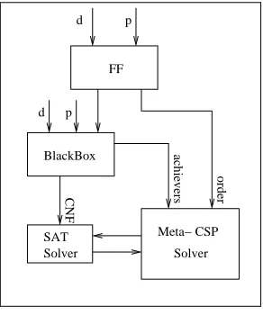
During this process, it is possible that the meta- CSP has assigned to all of its vari-ables but the SAT solver still has unassigned varivari-ables. In this case, the meta- CSP sub-mits to the default decision- making process of the SAT solver. When the SAT solver backtracks, it triggers a backtrack in the meta- CSP, so long as the decision backtracks as high as the last meta- CSP decision. Clearly, if the meta- CSP returns no solution, then there must be no solution since if no combination of potential goal achievers leads to a successful plan, there must be no plan. The complete architecture of the system is shown in Figure 1. The algorithm relies on three programs: the planner FF, a modified version of Blackbox that outputs both CNF and information about possible goal achiev-ers and a modified vachiev-ersion of the zChaff SAT solver, controlled by an added meta- CSP

solver. The planner provides an upper- bound,l, to plan down from, and a goal ordering.

Blackbox then calculates the CNF at lengthl, and separately outputs the variables that

represent:

– The potential final- achievers of each goal and

– the noops that would enforce a particular achieved goal until the end of the plan.

Then the meta- CSP solver orders its variables as they were achieved in the seed plan. It then solves the problem and returns the optimal plan.

4

Results

The following section describes the experimental setup to test the performance of the meta- CSP solver described in Section 3. All of the experiments are performed on a dual- core Intel Pentium D 3.40GHz desktop computer. The meta- CSP solver will be compared against the performance of Maxplan and Blackbox. The performance of each planner will be measured in time taken to solve each problem. The time is taken to be

user- time+system- time, and is limited to a total of 1800 seconds (half of one hour). Although the computer has 2GB of memory, the planners are limited to using 1.5GB. The justification behind this is that if a program approaches 2GB, then CPU usage drops significantly as the planner starts to swap memory. It then becomes very unlikely that either a plan will be returned or that the CPU time will timeout without an unreasonable wait.

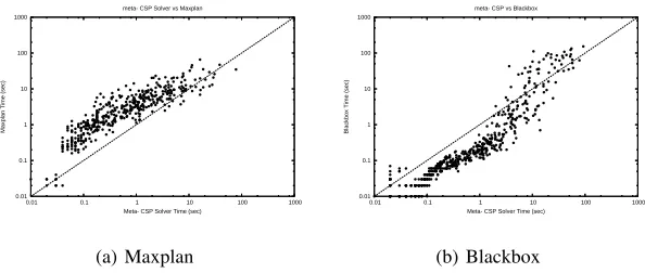
Blocksworld, Grid and Driverlog are the three domains that have been selected to test the meta- CSP solver. These will be described in the following sections. Graphs of the results for all of the problem instances are also shown. The graphs are log- scaled on both axes. Since the meta- CSP solver time is the x- axis and the competing planner

is the y- axis, any point plotted above the liney =xconstitutes a “win” for the

meta-CSP solver (as it denotes the competitor took a greater time). To ease the discernment

to the eye, the liney=xis also plotted.

4.1 Blocksworld

interesting structural properties and its simplicity. The form of Blocksworld studied in this work consists of a table on which any amount of stacks of blocks can be made. The initial state and goal state are two different configurations of the blocks, the problem is to rearrange the blocks into the goal configuration. The problem is clearly easy to satisfy: one approach could just be to unstack all of the blocks onto the table and then stack them into the goal configuration. However, solving the problem optimally is a difficult task.

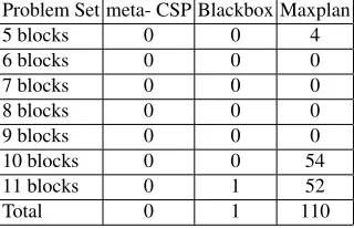
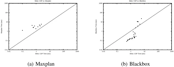
Using the problem generator of Thiebaux and Slaney [9], 100 random instances for each size of problem between 5 and 11 were generated, giving 700 instances in total. The results are shown in Figure 2(a) (Maxplan) and in Figure 2(b) (Blackbox). The numbers of unsolved instances are shown in Table 1.

0.01 0.1 1 10 100 1000

0.01 0.1 1 10 100 1000

Maxplan Time (sec)

meta- CSP Solver Time (sec) meta- CSP Solver vs Maxplan

(a) Maxplan

0.01 0.1 1 10 100 1000

0.01 0.1 1 10 100 1000

Blackbox Time (sec)

meta- CSP Solver Time (sec) meta- CSP Solver vs Blackbox

(b) Blackbox

Fig. 2.Combined blocksworld instances.

Problem Set meta- CSP Blackbox Maxplan

5 blocks 0 0 4

6 blocks 0 0 0

7 blocks 0 0 0

8 blocks 0 0 0

9 blocks 0 0 0

10 blocks 0 0 54

11 blocks 0 1 52

Total 0 1 110

4.2 Driverlog

Driverlog is a logistics style planning domain, first used in the 2002 International Plan-ning Competition. A Driverlog problem contains four types of object: locations, trucks, drivers and packages. Locations are connected by roads and paths. Drivers can walk along paths, whilst trucks can drive along roads. However, trucks cannot drive down paths, and drivers cannot walk in the road. Packages have to be transported in trucks, and trucks need to be driven by a driver in order to move anywhere. The typical goal in a Driverlog problem is to move a subset of all drivers, trucks and packages to some locations.

The problem set for the Driverlog domain is generated by a custom generator. This generator differs from the one used in the 2002 IPC in two major respects: it only generates planar graphs for the underlying maps and there is no extra location situ-ated between two locations joined by a path. These changes were made because planar graphs more realistically model a road network and the extra locations vastly increase the number of ground actions when walking actions are not often very important parts of Driverlog plans. The instances generated are all single driver, single truck problems with 15 locations. The parameter to be varied is the number of packages to be delivered. Each package, the driver and the truck each have a goal location, not equal to its start lo-cation. The number of packages is varied between 5 and 15, with 10 instances for each size. The results are shown in Figure 3(a) (Maxplan) and in Figure 3(b) (Blackbox). The numbers of unsolved instances are shown in Table 2.

0.01 0.1 1 10 100 1000

0.01 0.1 1 10 100 1000

Maxplan Time (sec)

Meta- CSP Time (sec) Meta- CSP vs. Maxplan

(a) Maxplan

0.01 0.1 1 10 100 1000

0.01 0.1 1 10 100 1000

Blackbox Time (sec)

Meta- CSP Time (sec) Meta- CSP vs. Blackbox

(b) Blackbox

Fig. 3.Combined Driverlog instances.

4.3 Grid

Problem Set meta- CSP Blackbox Maxplan

Driverlog 1 0 0 5

Driverlog 2 0 1 7

Driverlog 3 0 2 9

Driverlog 4 0 7 9

Driverlog 5 0 9 10

Driverlog 6 0 10 10

Driverlog 7 0 10 10

Driverlog 8 1 10 10

Driverlog 9 4 10 10

Driverlog 10 2 10 10

Driverlog 11 6 10 10

Driverlog 12 7 10 10

Driverlog 13 6 10 10

Driverlog 14 7 10 10

Driverlog 15 10 10 10

Total 43 119 140

Table 2.Numbers of failed instances in the Driverlog domain. The re are 10 problems in each problem set, making 150 in total.

is to be moved between locations. The cargo in Grid is a number of keys, and to get keys to their desired locations requires different locations to be unlocked. However, the key that unlocks a location may not be the key that needs to be delivered to that same location.

The Grid problem generator is supplied with the FF planning system [8]. The

pa-rameters of a Grid problem arex-dimension,y-dimension, number of keys (k#),

num-ber of locks (l#) and number of different types of key. Four different size grids will be

studied,3×3,3×4,4×4,4×5. In each of these sizes, there will be ten problems

generated for each of the following parameter sets:{(k#, l#)|k#∈ {1,2,3,4}, l#∈

{1,2,3,4}}giving 640 total instances. The results are shown in Figure 4(a) (Maxplan)

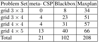
and in Figure 4(b) (Blackbox). The numbers of unsolved instances are shown in Table 3.

Problem Set meta- CSP Blackbox Maxplan

grid3×3 0 8 34

grid3×4 4 23 51

grid4×4 4 31 57

grid4×5 13 40 66

Total 21 102 208

0.01 0.1 1 10 100 1000

0.01 0.1 1 10 100 1000

Maxplan Time (sec)

Meta- CSP Solver Time (sec) meta- CSP Solver vs Maxplan

(a) Maxplan

0.01 0.1 1 10 100 1000

0.01 0.1 1 10 100 1000

Blackbox Time (sec)

Meta- CSP Solver Time (sec) meta- CSP vs Blackbox

(b) Blackbox

Fig. 4.Combined Grid instances.

5

Discussion

Comparing the meta- CSP solver and Maxplan is the best way to evaluate the per-formance of the meta- CSP model. This is because the major difference between the two planners is which model they use (meta- CSP or purely the SAT encoding). How-ever, for the sake of completeness, it is important to compare the results with another SAT planner. The comparison with Blackbox reveals some curious results, well wor-thy of discussion. These can provide some explanations of when it is better to use a forwards search direction and when to use a backwards search direction. When view-ing the graphs, it is important to consider how many problems were unsolved by each planner, as these points cannot be plotted.

5.1 Comparisons with Maxplan

The results were consistently better than those of Maxplan. In all three domains, the meta- CSP solver solves more instances that Maxplan. As shown in Table 1, Table 2 and

Table 3, of the 1490 instances, the meta- CSP solver solved 1426 (95.7%) compared to

the 458 (30.7%) that Maxplan solved. The graphs clearly show that, except for a few

that Maxplan solved. There are several of the harder instances in the Grid domain in which Maxplan performs better than the meta- CSP solver. Any indication that these points indicate that Maxplan is scaling better are unrealistic, however, considering the numbers of instances that remain unsolved by Maxplan.

The strongest results were gained in the Driverlog domain. The meta- CSP approach is suited to this domain because firstly, the goals are often achievable early in the plan (especially as the numbers of parcels increases). This means that the maintenance of the noops has an important impact on the planning process. Another reason the meta-CSP has an advantage is the fact that the schedule is tight. This means that once a final achiever is decided, propagation is more likely to lead to an outcome than if there was a lot of slack in the problem. Because these problems had only one truck and one achiever, the decision over resource allocation had already been decided, there was one choice.

As such, the scheduling decisions of when to deliver the packages was the key decision. This is demonstrated in the fact that the meta- CSP solver can solver larger, and more, instances than can Maxplan. In the Grid domain, other decisions that have no relation to the actual top- level goals are also important and so performance was closer.

5.2 Comparisons with Blackbox

As with Maxplan, Blackbox solved fewer instances than the meta- CSP solver. In total,

Blackbox solved 1268 of the 1490 problems. At 85.1%, that is still more than10%

fewer instances solved than the meta- CSP solver. As the graphs illustrate, however,

Blackbox usually performs better for the majority of thesolved instances. There are

several reasons that Blackbox performs better. There are overheads that searching in a backwards direction brings with it:

– Before search, the sub- optimal planner that is used to seed the plan has to solve

the problem. Although this is typically trivial, it can be an overhead on the total planning time, especially for simple problems, or problems that FF can perform badly on.

– Creating the SAT model is often the dominant part of the meta- CSP search time.

Because FF can often overestimate the optimal length greatly, twinned with the fact that in its current implementation, the meta- CSP solver is reliant on Blackbox

writing the model to disk (often creating CNF files>100MB), then just generating

the model can take a long time.

0.01 0.1 1 10 100 1000

0.01 0.1 1 10 100 1000

Blackbox Time (sec)

meta- CSP Solver Time (sec) meta- CSP Solver vs Blackbox

(a) 6 Blocks

0.01 0.1 1 10 100 1000

0.01 0.1 1 10 100 1000

Blackbox Time (sec)

meta- CSP Solver Time (sec) meta- CSP Solver vs Blackbox

(b) 8 Blocks

0.01 0.1 1 10 100 1000

0.01 0.1 1 10 100 1000

Blackbox Time (sec)

meta- CSP Solver Time (sec) meta- CSP Solver vs Blackbox

(c) 10 Blocks

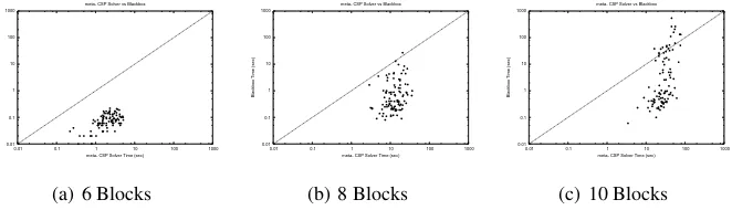
Fig. 5.Blocksworld instances partitioned by size.

The results for 6, 8 and 10 blocks are shown in Figure 5 and they reveal some in-triguing behaviour. The variance in the time it takes Blackbox to solve the instances seems to increase with the numbers of blocks, whereas the meta- CSP time seems to

remain more stable. With 10 blocks, Blackbox still solves many instances quickly (<1

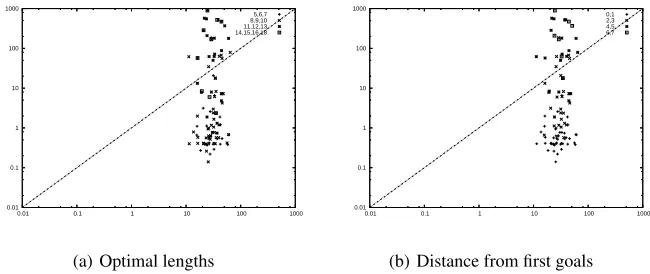
second), but others can take several hundred seconds. It seems somewhat intuitive that the meta- CSP solver might solve longer plans faster than Blackbox. This intuition coming from the fact that the meta- CSP solver begins with an overestimate, so a plan close to that estimate is better. The graph of the 11 block instances is plotted again in Figure 6(a), this time annotated with the optimal plan lengths, which range from 5 to 18 steps. To explain this result, it is necessary to also look at a different measure, the distance between the fist time the goals appear non- mutex in the planning- graph and the optimal plan length. This is shown in Figure 6(b). Notice that it is exactly those in-stances that are distant from the fixpoint, that the meta- CSP solver wins over Blackbox.

Only one instance that was in the6,7range was solved faster by Blackbox than by the

meta- CSP solver. In the previous range (4,5), the meta- CSP solver performs better

than Blackbox in 14 of 20 instances. There is a large cluster of results that Blackbox

solved in the range of0.1and1seconds that are all solvable either at, ar at the next

timepoint from, the time the goals first become reachable. So, it seems that problems that are solvable close to the level that the goals first become pairwise non- mutex are best solved by Blackbox, but the more distant problems are best solved by the meta-CSP solver.

0.01 0.1 1 10 100 1000

0.01 0.1 1 10 100 1000 5,6,7 8,9,10 11,12,13 14,15,16,18

(a) Optimal lengths

0.01 0.1 1 10 100 1000

0.01 0.1 1 10 100 1000 0,1 2,3 4,5 6,7

(b) Distance from first goals

Fig. 6.11 block annotated Blocksworld instances. The x- axes are the meta- CSP timings, the y-axes represent the Blackbox timings.

6

Related Work and Future Work

The idea of solving a problem using a Meta- CSP model was used in the BLUE

-BLOCKERsystem that optimally solves rectangle packing problems [10]. An interest-ing feature of this solver is that it models the rectangle packinterest-ing problem as a disjunctive temporal network, and each assignment in the meta- CSP represents the partial ordering of the rectangles to be packed. Only when a consistent partial ordering has been found, does the system attempt to find a concrete solution, though there may not be a valid solution even then.

Although competitive as a planner, there is clear space for development of the meta-CSP solver. The meta- meta-CSP solver currently has a variable ordering heuristic based on the order of which the goals are achieved on the seed plan. Currently the meta- CSP solver has no value ordering heuristic. Since the variables can have large domains (one goal can have many achievers), an ordering heuristic on the values could provide a performance increase. The meta- CSP model was motivated by the study of backdoors in planning problems. An observation being that the key scheduling decision of when to finally achieve a goal cannot be made explicitly in the SAT solver. The current solver searches across actual achieving actions of the goals. This means that decisions are also

being made abouthowgoals are achieved, and not justwhenthey are achieved. So, the

decisions that the meta- CSP is making are of a very course granularity. It may be that the key decisions regard mainly resource allocation, or scheduling, decisions. It has also been noted that some key decisions are allocation decisions that are completely unrelated to the goals (for instance, the keys in the Grid domain). The meta- CSP could

be altered such that variables represent this finer- grained structure, simplywhena goal

is achieved, orwhichresources are used in its achievement.

meta- CSP, and because the plan length is bounded, more landmarks could potentially be found.

7

Conclusions

We have introduced a novel reformulation of the planning problem. This is based on a constraint model that searches across the final achievers of the goals of the problem. We have shown this model to be competitive when compared to other state of the art SAT planners. It has been shown to solve more instances than both Maxplan and Blackbox across three domains: Blocksworld, Driverlog and Grid. Time performance is almost al-ways greater than Maxplan on the instances that Maxplan can solve. Often performance is worse than that of Blackbox, but it appears that this has much to do with the distance from the Graphplan fixpoint. Our analysis shows that the performance of Blackbox can degrade when plans are distant from the first time the goals appear non- mutex in the planning- graph. The results also demonstrate the fact that making the key scheduling decision of when to achieve a goal can improve the efficiency of search over a flat SAT model.

References

1. Helmert, M.: Complexity results for standard benchmark domains in planning. Artificial Intelligence143(2) (2003) 219–262

2. Helmert, M.: New complexity results for classical planning benchmarks. In: Proceedings of the Sixteenth International Conference on Automated Planning and Scheduling (ICAPS 2006). (2006) 52–61

3. Blum, A., Furst, M.: Fast planning through planning graph analysis. In: Proceedings of the 14th International Joint Conference on Artificial Intelligence (IJCAI 95). (1995) 1636–1642 4. Nebel, B., Dimopoulos, Y., Koehler, J.: Ignoring Irrelevant Facts and Operators in Plan Generation. In Steel, S., Alami, R., eds.: ECP. Volume 1348 of Lecture Notes in Computer Science., Springer (1997) 338–350

5. Long, D., Fox, M.: Efficient implementation of the plan graph in STAN. Journal of Artificial Intelligence Research10(1999) 87–115

6. Kautz, H.A., McAllester, D., Selman, B.: Encoding plans in propositional logic. In: Proceed-ings of the Fifth International Conference on the Principle of Knowledge Representation and Reasoning (KR’96). (1996) 374–384

7. Xing, Z., Chen, Y., Zhang, W.: Maxplan: Optimal planning by decomposed satisfiability and backward reduction. In: Proceedings of the Fifth International Planning Competition, International Conference on Automated Planning and Scheduling (ICAPS’06). (2006) 8. Hoffmann, J., Nebel, B.: The FF planning system: Fast plan generation through heuristic

search. Journal of Artificial Intelligence Research (JAIR)14(2001) 253–302

9. Slaney, J., Thiebaux, S.: Linear time near-optimal planning in the blocks world. In: Proceed-ings of the Thirteenth National Conference on Artificial Intelligence (AAAI-96), Portland, Oregon, USA, AAAI Press / The MIT Press (1996) 1208–1214

10. Moffitt, M.D., Pollack, M.E.: Optimal Rectangle Packing: A Meta-CSP Approach. In: In Proceedings of the 16th International Conference on Automated Planning and Scheduling. (2006) 93–102