The Zhou’s Method for Solving the Euler Equidimensional Equation

ISSN Online: 2152-7393 ISSN Print: 2152-7385

The Zhou’s Method for Solving the Euler

Equidimensional Equation

Pedro Pablo Cárdenas Alzate1_{, Jhon Jairo León Salazar}2_{, Carlos Alberto Rodríguez Varela}2 1_{Department of Mathematics and GEDNOL, Universidad Tecnológica de Pereira, Pereira, Colombia}

2_{Department of Mathematics, Universidad Tecnológica de Pereira, Pereira, Colombia}

Abstract

In this work, we apply the Zhou’s method [1] or differential transformation method (DTM) for solving the Euler equidimensional equation. The Zhou’s method may be considered as alternative and efficient for finding the approximate solutions of initial values problems. We prove superiority of this method by applying them on the some Euler type equation, in this case of order 2 and 3 [2]. The power series solution of the reduced equation transforms into an approximate implicit solution of the original equations. The results agreed with the exact solution obtained via transformation to a constant coefficient equation.

Keywords

Zhou’s Method, Equidimensional Equation, Euler Equation, DTM

1. Introduction

We know that when the coefficients p x

( )

and q x

( )

are analytic functions on a

given domain, then the equation y′′+ p x y

( )

′+q x y

( )

=0 has analytic fundamental

solution. We want to study equations with coefficients p and q having singularities, for this reason we study in this paper with one of the simplest cases, Euler’s equidimen- sional equation. This is an important problem because many differential equations in physical sciences have coefficients with singularities [3]. One of the special features of the equidimensional equation is that order of each derivative is equal to the power of the independent variable. This means that this type of equations can be reduced to linear equation with constant coefficient by using a change of the form x=et.

Many numerical methods were developed for this type of equations, specifically on Euler’s equations such that Laplace transform method and Adomian method [4]. The

How to cite this paper: Cárdenas Alzate, P.P., Salazar, J.J.L. and Varela, C.A.R. (2016) The Zhou’s Method for Solving the Euler Equidimensional Equation. Applied Ma-thematics, 7, 2165-2173.

http://dx.doi.org/10.4236/am.2016.717172 Received: September 15, 2016

Accepted: November 14, 2016 Published: November 17, 2016 Copyright © 2016 by authors and Scientific Research Publishing Inc. This work is licensed under the Creative Commons Attribution International License (CC BY 4.0).

http://creativecommons.org/licenses/by/4.0/

method proposed in this paper was first established by Zhou to solve problems in electric circuits analysis. In this work, the differential transformation method is applied to solver the Euler equidimensional equations and to illustrate this method, several equations of this type are solved [5][6].

2. The Euler Equidimensional Equation

A Euler equidimensional equation is a differential equation of the form

( )

1 2

1 2

1 1 2 2 1 0

d d d d

d

d d d

n n

n n

n n n n

y y y y

a x a x a x a x a y g x

x

x x x

− −

− −

+ +_+ + + = ₍₁₎

where an,,a0 are constants and d d n

n

y

x is an n-th derivative of the function y x

( )

and g x

( )

is a continuous function.

Now, we consider a second order differential equation (homogeneous Euler equidi- mensional) of the form

2 2 2 d d 0, 0 d d y y

ax bx cy x

x

x + + = > (2)

The solution can be obtained by using the change of variables

et

x= (3)

where d 1

d

t

x= x. In fact, for x>0, we introduce e

t

x= , therefore t=ln

( )

x . Then, the

first and second derivatives of y x

( )

are related by the chain rule,

2 2

2 2 2 2

d d d 1 d d d 1 d 1 d 1 d

and

d d d d d d d d d

y y t y y y y y

x t x x t x x x t x t x t

 

= = = _{ }= − +

  (4)

Now, substituting (4) in (2) yields a second order differential equation with constant coefficients, i.e.,

2 2

2 2

1 d d 1 d

0

d d

d

y y y

ax bx cy

t x t

x t   − + + =     2 2

d d d

0

d d

d

y y y

a a b cy

t t

t − + + =

(

)

2 2 d d 0 d d y y

a b a cy

t

t + − + = (5)

Equation (5) can be solved using the characteristic polynomial

(

)

2

0

am + b−a m+ =c (6)

where roots are m1 and m2 which give the general solution but depending on the

type of roots it has, i.e.,

a) If m1≠m2, real or complex, then the general solution of the Equation (2) is given

by

( )

1 2

1 2 , 1, 2 , 0

m m

y x =α x +α x α α ∈ x>

( )

1 1

( )

1 2 ln , 1, 2 , 0

m m

y x =α x +α x x α α ∈x>

3. The Zhou’s Method or DTM

Differential transformation method (DTM) of the function y x

( )

is defined as

( )

0

1 d ! d k

k x x

y Y k

k x ₌

 

= _{ }

  (7)

In (7), we have that y x

( )

is the original function and Y k

( )

is the transformed

function. The inverse differential transformation is defined as

( )

( )

0

, k

k

y x Y k x

∞

=

=

∑

(8)

but in real applications, function y x

( )

is expressed by a finite series and Equation (8)

can be written as

( )

( )

0

, n

k

k

y x Y k x

=

=

∑

₍₉₎

which implies that

( )

1 k

k n Y k x

∞

= +

∑

is negligibly small where n is decided by the convergence of natural frequency in this study.

The following theorems that can be deduced from Equations (7) and (9) and the proofs are available in [4][5][6].

Theorem 1 If y x

( )

= f x

( )

±g x

( )

, then Y k

( )

=F k

( )

±G x

( )

.

Theorem 2 If y x

( )

=α1f x

( )

, then Y k

( )

=α1F k

( )

with α1 constant.

Theorem 3 If

( )

d

d n

n

f y x

x

= _{, then}

( ) (

) ( )

!

!

k n

Y k F k n

k

+

= + _.

Theorem 4 If y x

( )

= f x g x

( ) ( )

, then

( )

( ) (

)

1 0 1 1

k k

Y k =

∑

₌F k G k−k .

Theorem 5 If

( )

n

y x =x , then Y k

( )

=δ

(

k−n

)

, where

(

)

1, 0,

k n

k n

k n

δ − _{= } =

≠ 

Theorem 6 (Cárdenas, P). If

( )

n

( )

y x =x f x , then

( )

0,

₍

₎

,

k n

Y k

F k n k n

< 

=  _{− ≥}



with n∈.

4. Numerical Results

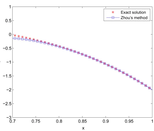
Example 1 (Homogeneous case). To begin, we consider the initial value problem

( )

( )

2

4 4 0

1 2, 1 11

x y xy y

y y

 ′′− ′+ =



 _′

= − = −

 (10)

Using the substitution (3) and (4), the IVP (10) is transformed to a second order differential equation with constant coefficients, i.e.,

( )

( )

(

)

( )

( )

2 2

1 1

4 4 0

x y t y t x y t y t

x x

 _{′′ − ′} ₋  _′ _{+ =}

   

   

( )

( )

4

( )

4

( )

0

y t′′ −y t′ − y t′ + y t =

( )

5

( )

4

( )

0

y t′′ − y t′ + y t = (11)

Now, of the initial conditions we have that as x=1, then t=0 and therefore

( )

0 2

y = − and y′

( )

0 = −11. So, the new IVP is given by

( )

( )

5 4 0

0 2, 0 11

y y y

y y

′′− ′+ = 

 _{= − ′ = −}

 (12)

The exact solution of the problem (12) is

( )

4 3

y x = −x x . Taking the differential

transformation of this problem we obtain

(

2 !

_{) ( ) ( ) ( ) ( )}

1 !

2 5 1 4 0

! !

k k

Y k Y k Y k

k k

+ +

+ − + + =

or

(

_{) ( )( ) ( ) ( ) ( )}

1

2 5 1 1 4

2 1

Y k k Y k Y k

k k

+ = _ + + − _

+ + (13)

where Y

( )

0 = −2 and Y

( )

1 = −11. Therefore, the recurrence Equation (13) gives:

• k=0,

( )

1

(

( )

( )

)

1

(

)

47

2 5 1 4 0 55 8

2 2 2

Y = Y − Y = − + = −

• k=1,

( )

1

(

( )

( )

)

1

(

)

191

3 10 2 4 1 235 44

6 6 6

Y = Y − Y = − + = −

• k=2,

( )

1

(

( )

( )

)

1 955 767

4 15 3 4 2 94

12 12 2 24

Y = Y − Y = _− + _= −

 

Therefore, using (9), the closed form of the solution can be easily written as

( )

( )

( )

( )

( )

2

( )

3

0

2 3 4

0 1 2 3

47 191 767 2 11

2 6 24

n k

k

y t Y k t Y Y t Y t Y t

t t t t

=

= = + + + +

= − − − − − −

∑





(14)

but since t=ln

( )

x , then we obtain (see Figure 1)

( )

( )

47

(

( )

)

2 191

(

( )

)

3 767

(

( )

)

4

2 11ln ln ln ln

2 6 24

[image:5.595.243.510.64.290.2]

Figure 1. The Zhou’s method vs. exact solution.

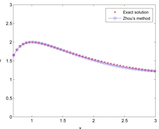
Example 2 (Non-homogeneous case). We consider the following IVP

( )

( )

( )

2

4 2 ln

1 2, 1 0

x y xy y x

y y

 ′′+ ′+ =



 _′

= =

 (15)

Then, problem (15) is transformed to a second order differential equation with con- stant coefficient by using (3) and (4), i.e.,

( )

( )

(

)

( )

( )

2 2

1 1

4 2

x y t y t x y t y t t

x x

 _{′′ − ′} ₊  _′ _{+ =}

   

   

( )

( )

4 ( ) 2

( )

y t′′ −y t′ + y t′ + y t =t

( )

3

( )

2

( )

y t′′ + y t′ + y t =t (16)

We know that of the initial conditions x=1 and therefore t=0, so we obtain

( )

0 2

y = and y′

( )

0 =0. Then, the IVP is given by

( )

( )

3 2

0 2, 0 0

y y y t

y y

′′+ ′+ = 

 _{= ′ =}

 (17)

The exact solution of the problem (15) is

( )

1 9 2 1

( )

3

5 ln

4 2 4

y x = x− − x− + x − . Now,

the DTM of (17) is

(

2 !

_{) ( ) ( ) ( ) ( ) ( )}

1 !

2 3 1 2 1

! !

k k

Y k Y k Y k k

k k δ

+ +

+ + + + = −

or

(

_{) ( )( ) ( ) ( ) ( ) ( )}

1

2 3 1 1 2 1

2 1

Y k k Y k Y k k

k k δ

+ = _− + + − + − _

+ + (18)

with Y

( )

0 =2 and Y

( )

1 =0. So, the recurrence Equation (18) gives:

( )

1

(

( )

( )

( )

)

1

( )

2 3 1 2 0 1 4 2

2 2

Y = − Y − Y +δ − = − = −

• k=1,

( )

1

(

( ) ( )

( )

( )

)

1

(

)

13

3 3 2 2 2 1 0 12 1

6 6 6

Y = − Y − Y +δ = + =

• k=2,

( )

1

(

( ) ( )

( )

( )

)

1 39 31

4 3 3 3 2 2 1 4

12 12 2 24

Y = − Y − Y +δ = _− + _= −

 

• k=3,

( )

1

(

( )

( )

( )

)

1 31 13 67

5 12 4 2 3 2

20 20 2 3 120

Y = − Y − Y +δ = _ − _=

 

Therefore, using (9), the closed form of the solution can be easily written as

( )

( )

( )

( )

( )

2

( )

3

0

2 3 4 5

0 1 2 3

13 31 67

2 0 2

6 24 120

n k

k

y t Y k t Y Y t Y t Y t

t t t t t

=

= = + + + +

= + − + − + +

∑





(19)

But since t=ln

( )

x , then we obtain (see Figure 2)

( )

(

( )

)

2 13

(

( )

)

3 35

(

( )

)

4 67

(

( )

)

5

2 2 ln ln ln ln

6 24 120

y x ≈ − x + x − x + x +

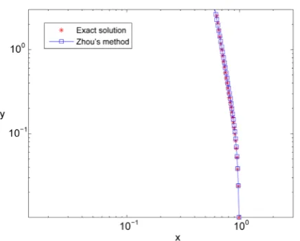
Example 3 (Third order Euler’s equation). Consider the following IVP

( )

( )

( )

3 2

10 20 20 0

1 0, 1 1, 1 1

x y x y xy y

y y y

 ′′′+ ′′− ′+ =



 _{′ ′′}

= = − =

 (20)

[image:6.595.241.512.466.686.2]

Now, to find y′′′

( )

x we use the chain rule. In fact we obtain

3 2 2 3 2

3 2 2 3 2 2 3 2

3 2

3 3 3 2 3

d d 1 d d 2 d d 1 1 d d

d d d

d d d d d

1 d 3 d 2 d

d

d d

y y y y y y y

x t t x

x x t x t x t t

y y y

t

x t x t x

       

=   − = −  − +   − 

     

   

= − +

(21)

Therefore, using (3), (4) and (21) we have

(

)

(

)

3 2

3 2

1 1 1

3 2 10 20 20 0

x y y y x y y x y y

x

x x

 _{′′′− ′′+ ′}₊  _{′′− ′}₋  _′_{+ =}

     

     

3 2 10 10 20 20 0

y′′′− y′′+ y′+ y′′− y′− y′+ y=

7 28 20 0

y′′′+ y′′− y′+ y= (22)

Now, as in the previous example x=1 and then t=0. So, the new initial con-

ditions are given by y

( )

0 =0,y′

( )

0 = −1 and y′′

( )

0 =1. Using (7) we find that

( )

0 0,

( )

1 1

Y = Y = − and

( )

2 1 2!

Y = . Therefore, we obtain the IVP

( )

( )

( )

7 28 20 0

0 0, 0 1, 0 1

y y y y

y y y

′′′+ ′′− ′+ = 

 _{= ′ = − ′′ =}

 (23)

Applying DTM to (23) we obtain

(

3 !

_{) ( ) ( ) ( ) ( ) ( )}

2 ! 1 !

_{( )}

3 7 2 28 1 20 0

! ! !

k k k

Y k Y k Y k Y k

k k k

+ + +

+ + + − + + =

or

(

)

(

)(

)(

)

(

)(

) (

)

(

) (

)

( )

3

1

7 2 1 2 28 1 1 20

3 2 1

Y k

k k Y k k Y k Y k

k k k

+

= _− + + + + + + − _

+ + +

(24)

So, the recurrence equation (24) gives:

• k=0,

( )

1

(

( ) ( )

( )

( )

)

1

(

)

35

3 7 2 2 28 1 20 0 7 28

6 6 6

Y = − Y + Y − Y = − − = −

• k=1,

( )

(

( )( ) ( )

( ) ( )

( )

)

( )

1

4 7 3 2 3 28 2 2 20 1

24

1 35 1 293

42 56 20 1

24 6 2 24

Y = − Y + Y − Y

 −    

= _− _{ }+ _{ }− − _=

   

 

• k=2,

( )

1

(

( )( ) ( )

( ) ( )

( )

)

5 7 4 3 4 28 3 3 20 2

60

1 293 35 1 1017

84 84 20

60 24 6 2 40

Y = − Y + Y − Y

   −    −

= _− _{ }+ _{ }− _{ }=

     

 

[image:8.595.266.485.66.242.2]

Figure 3. The Zhou’s method vs. exact solution.

( )

( )

( )

( )

( )

( )

( )

2 3

0

2 3 4 5

2 3 4 5

0 1 2 3

1 35 293 1017

0 1

2 6 24 40

1 35 293 1017

2 6 24 40

n k

k

y t Y k t Y Y t Y t Y t

t t t t t

t t t t t

=

= = + + + +

= + − + − + − +

= − + − + − +

∑



 

(25)

But since t=ln

( )

x , then we obtain (see Figure 3)

( )

(

( )

)

1

(

( )

)

2 35

(

( )

)

3 293

(

( )

)

4 1017

(

( )

)

5

ln ln ln ln ln

2 6 24 40

y x ≈ − x + x − x + x − x +

5. Conclusion

In this paper, we presented the definition and handling of one-dimensional differential transformation method or Zhou’s method. Using the substitutions (3) and (4), Euler’s equidimensional equations were transformed to a second and third order differential equations with constant coefficients, next using DTM these equations were transformed into algebraic equations (iterative equations). The new scheme obtained by using the Zhou’s method yields an analytical solution in the form of a rapidly convergent series. This method makes the solution procedure much more attractive. The figures [4][5]

and [6] clearly show the high efficiency of DTM with the three examples proposed.

Acknowledgements

Foremost, we would like to express my sincere gratitude to the Department of Mathe-matics of the Universidad Tecnológica de Pereira and group GEDNOL for the support in this work. In the same way, we would like to express sincere thanks to the anonym-ous reviewers for their positive and constructive comments towards the improvement of the article.

References

Huazhong University Press, Wuhan.

[2] Odibat, Z. (2008) Differential Transform Method for Solving Volterra Integral Equations with Separable Kernels. Mathematical and Computer Modelling, 48, 1144-1146.

http://dx.doi.org/10.1016/j.mcm.2007.12.022

[3] Shawagfeh, N. and Kaya, D. (2004) Comparing Numerical Methods for Solutions of Ordi-nary Differential Equations.Applied Mathematics Letters, 17, 323-328.

http://dx.doi.org/10.1016/S0893-9659(04)90070-5

[4] Ardila, W. and Cárdenas, P. (2013) The Zhou’s Method for Solving White-Dwarfs Equa-tion. Applied Mathematics, 10C, 28-32.

[5] Arikoglu, O. (2006) Solution of Difference Equations by Using Differential Transform Me-thod. Applied Mathematics and Computational, 173, 126-136.

[6] Cárdenas, P. and Arboleda, A. (2012) Resolución de ecuaciones diferenciales no lineales por el método de transformación diferencial. Universidad Tecnológica de Pereira, Colombia.

Tesis de Maestría en Matemáticas.

[7] Cárdenas, P. (2012) An Iterative Method for Solving Two Special Cases of Lane-Emden Type Equations. American Journal of Computational Mathematics, 4, 242-253.

Submit or recommend next manuscript to SCIRP and we will provide best service for you:

Accepting pre-submission inquiries through Email, Facebook, LinkedIn, Twitter, etc. A wide selection of journals (inclusive of 9 subjects, more than 200 journals)

Providing 24-hour high-quality service User-friendly online submission system Fair and swift peer-review system

Efficient typesetting and proofreading procedure

Display of the result of downloads and visits, as well as the number of cited articles Maximum dissemination of your research work

Submit your manuscript at: http://papersubmission.scirp.org/