Journal of Signal and Information Processing, 2016, 7, 227-251 http://www.scirp.org/journal/jsip ISSN Online: 2159-4481 ISSN Print: 2159-4465
Inspection of the Output of a Convolution and
Deconvolution Process from the Leading Digit
Point of View—Benford’s Law
Monika Pinchas
Department of Electrical and Electronic Engineering Ariel University, Ariel, Israel
Abstract
In the communication field, during transmission, a source signal undergoes a con-volutive distortion between its symbols and the channel impulse response. This dis-tortion is referred to as Intersymbol Interference (ISI) and can be reduced signifi-cantly by applying a blind adaptive deconvolution process (blind adaptive equalizer) on the distorted received symbols. But, since the entire blind deconvolution process is carried out with no training symbols and the channel’s coefficients are obviously unknown to the receiver, no actual indication can be given (via the mean square er-ror (MSE) or ISI expression) during the deconvolution process whether the blind adaptive equalizer succeeded to remove the heavy ISI from the transmitted symbols or not. Up to now, the output of a convolution and deconvolution process was mainly investigated from the ISI point of view. In this paper, the output of a convolution and deconvolution process is inspected from the leading digit point of view. Simulation results indicate that for the 4PAM (Pulse Amplitude Modulation) and 16QAM (Qu-adrature Amplitude Modulation) input case, the number “1” is the leading digit at the output of a convolution and deconvolution process respectively as long as heavy ISI exists. However, this leading digit does not follow exactly Benford’s Law but fol-lows approximately the leading digit (digit 1) of a Gaussian process for independent identically distributed input symbols and a channel with many coefficients.
Keywords
Blind Adaptive Equalizers, Blind Adaptive Deconvolution, Leading Digit Theory, Benford’s Law
1. Introduction
We consider a blind deconvolution problem in which we observe the output of an
un-How to cite this paper: Pinchas, M. (2016) Inspection of the Output of a Convolution and Deconvolution Process from the Lead-ing Digit Point of View—Benford’s Law. Journal of Signal and Information Processing, 7, 227-251.
http://dx.doi.org/10.4236/jsip.2016.74020 Received: September 8, 2016
Accepted: November 19, 2016 Published: November 22, 2016 Copyright © 2016 by author and Scientific Research Publishing Inc. This work is licensed under the Creative Commons Attribution International License (CC BY 4.0).
http://creativecommons.org/licenses/by/4.0/
known, possibly nonminimum phase, linear system (single-input-single-output (SISO) finite impulse response (FIR) system) from which we want to recover its input (source) using an adjustable linear filter (equalizer). During transmission, a source signal un-dergoes a convolutive distortion between its symbols and the channel impulse response. This distortion is referred to as ISI [1] [2] [3]. It is well known that ISI is a limiting fac-tor in many communication environments where it causes an irreducible degradation of the bit error rate thus imposing an upper limit on the data symbol rate [1] [4]. In order to overcome the ISI problem, a blind adaptive equalizer can be implemented in those systems [2]-[26]. But, since no training symbols are used in the deconvolution process and the channel coefficients are unknown to the receiver, no indication can be made (via the ISI or MSE expressions) during the deconvolution process whether the blind adaptive equalizer succeeded to remove the heavy ISI from the transmitted sym-bols or not. Such an information can be very useful to those systems involving the va-riable step-size parameter technique to get on one hand a fast removal of the heavy ISI by applying initially a relative high valued step-size parameter and then continuing with another step-size parameter which is lower compared to the first one in order to achieve on the other hand a very low residual ISI at the latter stages of the deconvolu-tion process [27]-[30].
According to [31], Benfords law (also known as the first-digit law) defines a peculiar distribution of the leading digits of a set of numbers. The behavior is logarithmic, with the leading digit 1 reflecting largest probability of occurrence and the remaining ones showing decreasing probabilities of appearance following a logarithmic trend. Accord-ing to [31], Benfords law has been widely proposed as a discriminatAccord-ing tool for natural-ly-shaped datasets [32] and even employed [33] or criticized [34] as a somewhat reliable diagnostic tool to detect a large variety of frauds. In [31], Benfords law was evaluated as a discriminator for audio signals. In particular it was employed to detect differences between natural and artificially created chords and real music.
In the communication field, the transmitted symbols may belong to a squared con-stellation input such as the 16QAM or to a PAM concon-stellation where the transmitted symbols are statistically independent and have the same probability to appear for transmission. Thus, the recovered symbols should also appear approximately with equal probability. Up to now, the output of a convolution process such as the output of a channel was mainly investigated from the ISI point of view. In this paper, the output of a convolution and deconvolution process is inspected from the leading digit point of view. Simulation results will indicate that for the 4PAM and 16QAM constellation in-put, the number 1 is the leading digit at the output of a convolution and deconvolution process respectively as long as heavy ISI exists. However, this leading digit does not follow exactly Benford’s Law but follows approximately the leading digit (digit 1) of a Gaussian process for independent identically distributed input symbols and a channel with many coefficients.
M. Pinchas
process from the leading digit point of view is given via simulation results in Section 3. Section 4 is our conclusion.
2. System Description
The system under consideration is illustrated in Figure 1, where we make the following assumptions:
1) The input sequence x n
[ ]
belongs to a 16QAM input constellation (a modulation using ± {1, 3} levels for in-phase and quadrature components) or a 4PAM case (a modulation using ± {1, 3} levels for the symbols) with variance 2x
σ
where x nr[ ]
and[ ]
i
x n are the real and imaginary parts of x n
[ ]
respectively. The input symbols are independent and identically distributed.2) The unknown channel h n
[ ]
is a possibly nonminimum phase linear time-in- variant filter in which the transfer function has no “deep zeros”, namely, the zeros lie sufficiently far from the unit circle.3) The equalizer c n
[ ]
is a tap-delay line.4) The noise w n
[ ]
is an additive Gaussian white noise with zero mean and variance[ ] [ ]
2
w E w n w n
σ ∗
= where E
[ ]
⋅ is the expectation operator and( )
⋅∗ is the conju-gate operation on
( )
⋅ .The transmitted sequence x n
[ ]
is sent via the channel h n[ ]
where it is also cor- rupted with noise w n[ ]
. Thus, the equalizer’s input sequence y n[ ]
may be written as:[ ] [ ] [ ] [ ]
y n =x n h n w n∗ + (1) where “∗” denotes the convolution operation. The equalized output sequence is defined by:
[ ] [ ] [ ] [ ] [ ] [ ]
z n = y n c n∗ =x n +p n w n+ (2) where p n
[ ]
is the convolutional noise (convolutional error) due to non-ideal equalizer’s coefficients (h n c n[ ] [ ] [ ]
∗ ≠δ
n ) and w n[ ]
=w n c n[ ] [ ]
∗ . Next, we turn to the mathe- matical definition of the ISI expression:2 2
max 2 max
m
m s s
ISI
s −
=
∑
(3)
where smax is the component of s, given by s c n h n=
[ ] [ ]
∗ , having the maximalabsolute value. Now, we turn to the adaptation mechanism of the equalizer’s coefficients which is based in this paper on Godard’s method [5] (a cost function approach):
[
]
[ ]
[ ]
[ ]
[ ]
[ ] [
]
4 2 * 2 1 m mE x n
c n c n z n z n y n m
E x n µ + = − − − (4)
where µ is the step-size parameter, ⋅ is the absolute value of
( )
⋅ ,(
)
0,1,2, , 1
m= N− and N is the equalizer’s tap length. Please note that we could use here for the blind adaptive deconvolution method any other cost function approach like the one given in [6] [9] [10] [12] [13] [20] or [24] for instance as well as just using the Bayesian technique as was done in [4] [17] [21] [22] and [26]. Next, we introduce Benford’s Law. According to [31], the probability value of the d-th digit is computed as follows:
( )
log 110 1P d
d
= +
(5) where d is the digit number.
3. The Output of a Convolution and Deconvolution Process from
the Leading Digit Point of View
In this section we first start to inspect the output of the convolution process from the leading digit point of view for the noiseless case. After that, we turn to inspect the output of the deconvolution process considering also the noisy situation.
In the following we use the 4PAM constellation input with three different channel cases having real valued coefficients:
Case I: Rayleigh fading channel with variance equal to 0.2. Case II: Gaussian channel with zero mean and variance equal to 1.
Case III: A channel where the coefficients are uniformly distributed within
[
− +1, 1]
. Figures 2-8 show the averaged value for the leading-digit distribution for 9000 symbolsM. Pinchas
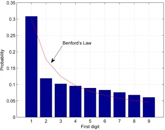
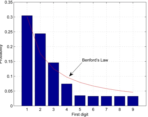
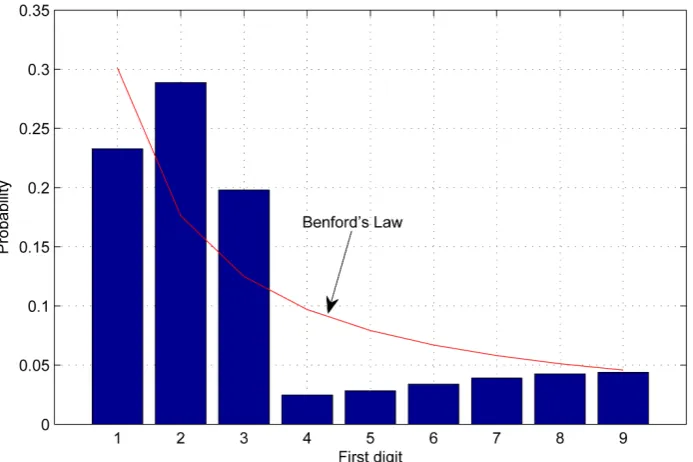
Figure 3. The leading-digit distribution for 9000 symbols (4PAM constellation) sent via a Rayleigh channel compared to Benford’s law. The channel length was set to 23. The averaged results were obtained in 100 Monte Carlo trials for the noiseless case.
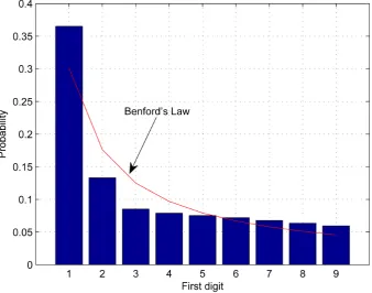
Figure 5. The leading-digit distribution for 9000 symbols (4PAM constellation) sent via a Rayleigh channel compared to Benford’s law. The channel length was set to 53. The averaged results were obtained in 100 Monte Carlo trials for the noiseless case.
M. Pinchas
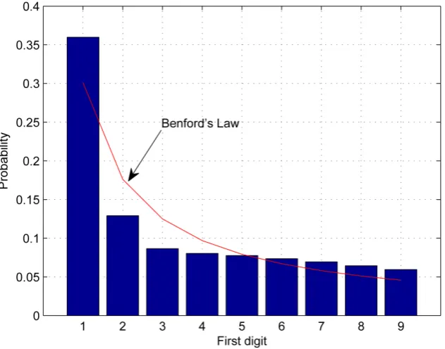
Figure 7. The leading-digit distribution for 9000 symbols (4PAM constellation) sent via the channel compared to Benford’s law. The channel’s coefficients were uniformly distributed within
[
− +1, 1]
. The channel length was set to 13. The averaged results were obtained in 100 MonteCarlo trials for the noiseless case.
Figure 8. The leading-digit distribution for 9000 symbols (4PAM constellation) sent via the channel compared to Benford’s law. The channel’s coefficients were uniformly distributed within
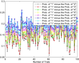
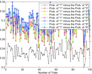
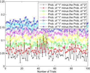
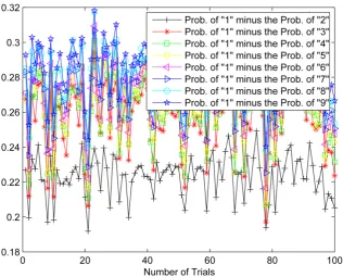
[image:7.595.216.536.393.648.2](belonging to a 4PAM constellation) sent via the above mentioned channel cases with different values for the channel length, compared with Benford’s law. 100 Monte Carlo trials were used to get the averaged results for the leading-digit distribution for each channel case and channel length, where for each trial, the channel coefficients were randomly selected from the predefined channel case. According to Figures 2-8, the leading digit at the output channel is the number 1. This phenomenon becomes even more evident for higher values for the channel length (Figure 5, Figure 8). Although the number 1 is the leading digit at the output channel (Figures 2-8), this leading digit (number 1) does not follow Benford’s law as it can be seen according to Figures 2-8. Figure 9 shows the averaged value for the leading-digit distribution for 9000 numbers belonging to a Gaussian distribution with zero mean and variance 1 compared to Benford’s law. According to Figure 9, the number 1 is the leading digit but it does not follow Benford’s law. Based on the central limit theorem [35], the output channel can be approximately considered as Gaussian for a high valued channel length. Therefore, the leading digit (number 1) behavior in Figure 5 and Figure 8 is similar to that obtained in Figure 9. Figures 2-8 show averaged results of the leading digit distribution. Therefore, in order to show that the leading number is 1 for each simulation trial out of the 100 Monte Carlo trials, further simulation was set up. Figures 10-16 show the probability of occurrence of the number 1 minus the probability of occurrence of the number “i” (where i=2,3, 4, ,9 ) for each trial out of the 100
[image:8.595.218.534.416.664.2]Monte Carlo trials valid for the above mentioned channel cases and different values for the channel length. According to Figures 10-16, the probability of occurrence of the
M. Pinchas
Figure 10. Probability of occurrence of the number 1 minus the probability of occurrence of the number “i” (where i=2,3,4, ,9 ) for each trial out of the 100 Monte Carlo trials. The results were obtained by sending 9000 symbols (4PAM constellation) via channel case I where the channel length was set to 13.
[image:9.595.214.533.397.651.2]Figure 12. Probability of occurrence of the number 1 minus the probability of occurrence of the number “i” (where i=2,3,4, ,9 ) for each trial out of the 100 Monte Carlo trials. The results were obtained by sending 9000 symbols (4PAM constellation) via channel case I where the channel length was set to 33.
[image:10.595.215.533.395.651.2]M. Pinchas
Figure 14. Probability of occurrence of the number 1 minus the probability of occurrence of the number “i” (where i=2,3,4, ,9 ) for each trial out of the 100 Monte Carlo trials. The results were obtained by sending 9000 symbols (4PAM constellation) via channel II where the channel length was set to 13.
[image:11.595.216.533.396.651.2]Figure 16. Probability of occurrence of the number 1 minus the probability of occurrence of the number “i” (where i=2,3,4, ,9 ) for each trial out of the 100 Monte Carlo trials. The results were obtained by sending 9000 symbols (4PAM constellation) via channel case III where the channel length was set to 53.
number 1 minus the probability of occurrence of the number “i” (where 2,3, 4, ,9
i= ) is higher than zero for each trial out of the 100 Monte Carlo trials.
Thus, according to Figures 10-16, the leading digit is the number 1.
Now, we turn to the deconvolution case where the equalized output is of our interest. 9000 symbols belonging to a 16QAM input constellation were sent via the channel used in [20]:
(
0 for 0; 0.4 for 0; 0.84 0.4 forn1 0)
n
h = n< − n= ⋅ − n> .
M. Pinchas
Figure 17. The leading-digit distribution at the equalized output compared to Benford’s law. The channel length as well as the equalizer’s tap length were set to 13. The step-size parameter was set to 0.00008. The averaged results were obtained in 100 Monte Carlo trials for SNR=30 dB. After 10 iterations the averaged residual ISI reached −3.75 dB and at that level of the residual ISI the equalizer’s coefficients were not updated anymore.
[image:13.595.219.533.401.649.2]Figure 19. The leading-digit distribution at the equalized output compared to Benford’s law. The channel length as well as the equalizer’s tap length were set to 13. The step-size parameter was set to 0.00008. The averaged results were obtained in 100 Monte Carlo trials for SNR=30 dB. The
averaged residual ISI was −14 dB after 500 iterations.
[image:14.595.206.550.378.648.2]M. Pinchas
[image:15.595.233.513.142.372.2]not follow Benford’s law. According to Figure 19 and Figure 20 the number 1 is no more the leading digit at the equalized output. Thus, this may indicate that most of the ISI is already removed by the equalizer which is confirmed in our case with Figure 21 and Figure 22. Figures 23-26 show the probability of occurrence of the number 1
Figure 21. The real part of the equalized output for SNR=30 dB. The channel length as well as the equalizer’s tap length were set to 13. The step-size parameter was set to 0.00008. The averaged residual ISI was −14 dB after 500 iterations.
[image:15.595.237.511.434.661.2]Figure 23. Probability of occurrence of the number 1 minus the probability of occurrence of the number “i” (where i=2,3,4, ,9 ) for each trial out of the 100 Monte Carlo trials obtained at the equalized output for SNR=30 dB. The channel length as well as the equalizer’s tap length were set to 13. The step-size parameter was set to 0.00008. The averaged residual ISI was −3.75 dB after 10 iterations.
Figure 24. Probability of occurrence of the number 1 minus the probability of occurrence of the number “i” (where i=2,3,4, ,9 ) for each trial out of the 100 Monte Carlo trials obtained at the equalized output for SNR=30 dB. The channel length as well as the equalizer’s tap length were
[image:16.595.227.523.397.637.2]M. Pinchas
Figure 25. Probability of occurrence of the number 1 minus the probability of occurrence of the number “i” (where i=2,3,4, ,9 ) for each trial out of the 100 Monte Carlo trials obtained at the equalized output for SNR=30 dB. The channel length as well as the equalizer’s tap length were
set to 13. The step-size parameter was set to 0.00008. The averaged residual ISI was −14 dB after 500 iterations.
Figure 26. Probability of occurrence of the number 1 minus the probability of occurrence of the number “i” (where i=2,3,4, ,9 ) for each trial out of the 100 Monte Carlo trials obtained at the equalized output for SNR=30 dB. The channel length as well as the equalizer’s tap length were
[image:17.595.223.524.395.634.2]minus the probability of occurrence of the number “i” (where i=2,3, 4, ,9 ) for each trial out of the 100 Monte Carlo trials valid at the equalized output for SNR of 30 dB. Since the transmitted symbols were sent statistically independent with the same probability to appear, the recovered symbols should also appear approximately with equal probability. Indeed, according to Figures 23-26, the probability of occurrence of the number 1 minus the probability of occurrence of the number 3 is approximately zero only at the latter stages of the deconvolution process (Figure 25, Figure 26) while this is not the case at the earlier stages of the deconvolution process (Figure 23, Figure 24). Please note that according to Figure 24, the number 1 was not the leading number for the entire 100 Monte Carlo trials. This outcome can be explained by the fact that the residual ISI was probably much lower than the averaged residual ISI of −7.5 dB. Thus, the system was closer to the symbol recovery state. Next, we turn to the SNR=20 dB case. Figures 27-29 show the averaged value for the leading-digit distribution at the equalized output for SNR of 20 dB compared with Benford’s law. As it was for the case of SNR=30 dB, the number 1 is the leading digit at the equalized output at the early stages of the deconvolution process (Figure 27). According to Figure 28 and Figure 29 the number 1 is no more the leading digit at the equalized output. Thus, this may indicate that most of the ISI is already removed by the equalizer which is confirmed in our case with Figure 30 and Figure 31. In addition, the leading digit (number 1) does not follow Benford’s law (Figure 27). Figures 32-34 show the probability of occurrence of the number 1 minus the probability of occurrence of the number “i” (where
2,3, 4, ,9
[image:18.595.222.531.411.648.2]i= ) for each trial out of the 100 Monte Carlo trials valid at the equalized
M. Pinchas
Figure 28. The leading-digit distribution at the equalized output compared to Benford’s law. The channel length as well as the equalizer’s tap length were set to 13. The step-size parameter was set to 0.00008. The averaged results were obtained in 100 Monte Carlo trials for SNR=20 dB. The
averaged residual ISI was −11.5 dB after 400 iterations.
[image:19.595.216.537.395.648.2]Figure 30. The real part of the equalized output for SNR=20 dB. The channel length as well as the equalizer’s tap length were set to 13. The step-size parameter was set to 0.00008. The averaged residual ISI was −11.5 dB after 400 iterations.
[image:20.595.213.535.398.662.2]M. Pinchas
Figure 32. Probability of occurrence of the number 1 minus the probability of occurrence of the number “i” (where i=2,3,4, ,9 ) for each trial out of the 100 Monte Carlo trials obtained at the equalized output for SNR=20 dB. The channel length as well as the equalizer’s tap length were
set to 13. The step-size parameter was set to 0.00008. The averaged residual ISI was −3.75 dB after 10 iterations.
Figure 33. Probability of occurrence of the number 1 minus the probability of occurrence of the number “i” (where i=2,3,4, ,9 ) for each trial out of the 100 Monte Carlo trials obtained at the equalized output for SNR=20 dB. The channel length as well as the equalizer’s tap length were
[image:21.595.224.525.398.638.2]Figure 34. Probability of occurrence of the number 1 minus the probability of occurrence of the number “i” (where i=2,3,4, ,9 ) for each trial out of the 100 Monte Carlo trials obtained at the equalized output for SNR=20 dB. The channel length as well as the equalizer’s tap length were set to 13. The step-size parameter was set to 0.00008. The averaged residual ISI was −16.5 dB after 800 iterations.
output for SNR of 20 dB. According to Figures 32-34, the probability of occurrence of the number 1 minus the probability of occurrence of the number 3 is approximately zero only at the latter stages of the deconvolution process (Figure 34) while this is not the case at the earlier stages of the deconvolution process (Figure 32).
4. Conclusion
In this paper, we have shown via simulation results that the number 1 is the leading digit at the output of a convolution and deconvolution process for a 4PAM and 16QAM input constellation respectively, as long as heavy ISI exists. In addition, simulation results have shown that the behaviour of this leading digit does not follow exactly Benford’s Law but follows approximately the leading digit (digit 1) of a Gaussian process for independent identically distributed input symbols and a channel with many coefficients.
Acknowledgements
We thank the Editor and the referee for their comments.
References
[1] Pinchas, M. (2013) Residual ISI Obtained by Nonblind Adaptive Equalizers and Fractional Noise. Mathematical Problems in Engineering, 2013, Article ID: 830517.
M. Pinchas
[2] Pinchas, M. (2013) Two Blind Adaptive Equalizers Connected in Series for Equalization Performance Improvement. Journal of Signal and Information Processing, 4, 64-71.
http://dx.doi.org/10.4236/jsip.2013.41008
[3] Pinchas, M. (2013) Residual ISI Obtained by Blind Adaptive Equalizers and Fractional Noise. Mathematical Problems in Engineering, 2013, Article ID: 972174.
http://dx.doi.org/10.1155/2013/972174
[4] Pinchas, M. and Bobrovsky, B.Z. (2006) A Maximum Entropy Approach for Blind Decon-volution. Signal Processing, 86, 2913-2931. http://dx.doi.org/10.1016/j.sigpro.2005.12.009
[5] Godard, D.N. (1980) Self Recovering Equalization and Carrier Tracking in Two-Dime- nional Data Communication System. IEEE Transactions on Communications, 28, 1867- 1875. http://dx.doi.org/10.1109/TCOM.1980.1094608
[6] Lazaro, M., Santamaria, I., Erdogmus, D., Hild, K.E., Pantaleon, C. and Principe, J.C. (2005) Stochastic Blind Equalization Based on PDF Fitting Using Parzen Estimator. IEEE Transac-tions on Signal Processing, 53, 696-704. http://dx.doi.org/10.1109/TSP.2004.840767
[7] Sato, Y. (1975) A Method of Self-Recovering Equalization for Multilevel Amplitude-Mod- ulation Systems. IEEE Transactions on Communications, 23, 679-682.
http://dx.doi.org/10.1109/TCOM.1975.1092854
[8] Beasley, A. and Cole-Rhodes, A. (2005) Performance of an Adaptive Blind Equalizer for QAM Signals. IEEE Military Communications Conference, Atlantic City, 17-20 October 2005, 2373-2377. http://dx.doi.org/10.1109/milcom.2005.1606023
[9] Alaghbari, K.A.A., Tan, A.W.C. and Lim, H.S. (2012) Cost Function of Blind Channel Equalization. 4th International Conference on Intelligent and Advanced Systems (ICIAS), Kuala Lumpur, 12-14 June 2012, 665-669. http://dx.doi.org/10.1109/icias.2012.6306097
[10] Daas, A., Hadef, M. and Weiss, S. (2009) Adaptive Blind Multiuser Equalizer Based on PDF Matching. International Conference on Telecommunications (ICT), Marrakech, 25-27 May 2009, 213-216. http://dx.doi.org/10.1109/ictel.2009.5158646
[11] Giunta, G. and Benedetto, F. (2013) A Signal Processing Algorithm for Multi-Constant Modulus Equalization. 36th International Conference on Telecommunications and Signal Processing (TSP), Rome, 2-4 July 2013, 52-56. http://dx.doi.org/10.1109/TSP.2013.6613890
[12] Daas, A. and Weiss, S. (2010) Blind adaptive Equalizer Based on PDF Matching for Ray-leigh Time-Varying Channels. Conference Record of the 44th Asilomar Conference on Signals, Systems and Computers (ASILOMAR), Pacific Grove, 7-10 November 2010, 456- 460. http://dx.doi.org/10.1109/acssc.2010.5757600
[13] Abrar, S. (2005) A New Cost Function for the Blind Equalization of Cross-QAM Signals. 17th International Conference on Microelectronics (ICM 2005), Islamabad, 13-15 Decem-ber 2005, 290-295. http://dx.doi.org/10.1109/icm.2005.1590087
[14] Blom, K.C.H., Gerards, M.E.T., Kokkeler, A.B.J. and Smit, G.J.M. (2013) Nonminimum- Phase Channel Equalization Using All-Pass CMA. 24th International Symposium on Per-sonal Indoor and Mobile Radio Communications (PIMRC), London, 8-9 September 2013, 1467-1471. http://dx.doi.org/10.1109/pimrc.2013.6666373
[15] Nikias, C.L. and Petropulu, A.P. (Eds.) (1993) Higher-Order Spectra Analysis: A Nonlinear Signal Processing Framework. Prentice-Hall, Upper Saddle River, Chapter 9, 419-425. [16] Bellini, S. (1986) Bussgang Techniques for Blind Equalization. IEEE Global
Telecommuni-cation Conference Records, Houston, 1-4 December 1986, 1634-1640.
[17] Fiori, S. (2001) A Contribution to (Neuromorphic) Blind Deconvolution by Flexible Ap-proximated Bayesian Estimation. Signal Processing, 81, 2131-2153.
[18] Haykin, S. (1991) Blind Deconvolution. In: Haykin, S., Ed., Adaptive Filter Theory, Pren-tice-Hall, Englewood Cliffs, Chapter 20.
[19] Pinchas, M. (2010) A Closed Approximated Formed Expression for the Achievable Residual Intersymbol Interference Obtained by Blind Equalizers. Signal Processing Journal, 90, 1940-1962. http://dx.doi.org/10.1016/j.sigpro.2009.12.014
[20] Shalvi, O. and Weinstein, E. (1990) New Criteria for Blind Deconvolution of Nonminimum Phase Systems (Channels). IEEE Transactions on Information Theory, 36, 312-321.
http://dx.doi.org/10.1109/18.52478
[21] Pinchas, M. (2011) 16QAM Blind Equalization Method via Maximum Entropy Density Approximation Technique. International Conference on Signal and Information Processing
(CSIP), Shanghai, 28-30 October 2011, 700-703.
http://wenku.baidu.com/view/30d075b569dc5022aaea002a.html
[22] Pinchas, M. and Bobrovsky, B.Z. (2007) A Novel HOS Approach for Blind Channel Equali-zation. IEEE Transactions on Wireless Communications, 6, 875-886.
http://dx.doi.org/10.1109/TWC.2007.04404
[23] Gitlin, R.D., Hayes, J.F. and Weinstein, S.B. (1992) Automatic and Adaptive Equalization. In: Gitlin, R.D., Hayes, J.F. and Weinstein, S.B., Eds., Data Communications Principles, Plenum, New York, 517-605. http://dx.doi.org/10.1007/978-1-4615-3292-7
[24] Pinchas, M. (2011) A MSE Optimized Polynomial Equalizer for 16QAM and 64QAM Con-stellation. Signal, Image and Video Processing, 5, 29-37.
http://dx.doi.org/10.1007/s11760-009-0138-z
[25] Im, G.-H., Park, C.J. and Won, H.C. (2001) A Blind Equalization with the Sign Algorithm for Broadband Access. IEEE Communications Letters, 5, 70-72.
http://dx.doi.org/10.1109/4234.905939
[26] Pinchas, M. (2016) New Lagrange Multipliers for the Blind Adaptive Deconvolution Prob-lem Applicable for the Noisy Case. Entropy, 18, 65. http://dx.doi.org/10.3390/e18030065
[27] Demir, M.A. and Ozen, A. (2012) A Novel Variable Step Size Adjustment Method Based on Autocorrelation of Error Signal for the Constant Modulus Blind Equalization Algorithm.
Radioengineering, 21, 37-45.
[28] Hamzehyan, R., Dianat, R. and Shirazi, N.C. (2012) New Variable Step-Size Blind Equaliza-tion Based on Modified Constant Modulus Algorithm. International Journal of Machine Learning and Computing, 2, 30-34. http://dx.doi.org/10.7763/IJMLC.2012.V2.85
[29] Xiong, Z., Li, L., Zhuo, D., Dong, Z. and Zhang, L. (2004) A New Adaptive Step-Size Blind Equalization Based on Autocorrelation of Error Signal. 7th International Conference on Signal Processing, 2, 1719-1722.
[30] Iyi, Z., Lei, C. and Yunshan, S. (2009) Variable Step-Size CMA Blind Equalization Based on Non-Linear Function of Error Signal. International Conference on Communications and Mobile Computing, 1, 396-399.
[31] Barbancho, I., Tardon, L.J., Barbancho, A.M. and Sbert, M. (2015) Benford’s Law for Music Analysis. Proceedings of the 16th ISMIR Conference, Malaga, Spain, 26-30 October 2015, 735-741.
[32] Del Acebo, E. and Sbert, M. (2005) Benford’s Law for Natural and Synthetic Images. Pro-ceedings of the 1st Eurographics Conference on Computational Aesthetics in Graphics, Vi-sualization and Imaging, Girona, 18-20 May 2005, 169-176.
[33] Jacob, B.A. and Levitt, S.D. (2003) Rotten Apples: An Investigation of the Prevalence and Predictors of Teacher Cheating. The Quarterly Journal of Economics, 118, 843-877.
M. Pinchas
[34] Deckert, J., Myagkov, M. and Ordeshook, P.C. (2010) The Irrelevance of Benford’s Law for Detecting Fraud in Elections. Caltech/MIT Voting Technology Project,Working Paper. [35] Papoulis, A. (1965) Probability, Random Variables, and Stochastic Processes. International
Student Edition, McGraw-Hill, New York, Chapter 8, 266.
Abbreviations
ISI: Intersymbol Interference SNR: Signal to Noise Ratio SISO: Single Input Single Output FIR: Finite Impulse Response
QAM: Quadrature Amplitude Modulation PAM: Pulse Amplitude Modulation
Submit or recommend next manuscript to SCIRP and we will provide best service for you:
Accepting pre-submission inquiries through Email, Facebook, LinkedIn, Twitter, etc. A wide selection of journals (inclusive of 9 subjects, more than 200 journals)
Providing 24-hour high-quality service User-friendly online submission system Fair and swift peer-review system
Efficient typesetting and proofreading procedure
Display of the result of downloads and visits, as well as the number of cited articles Maximum dissemination of your research work
Submit your manuscript at: http://papersubmission.scirp.org/