Provincial Technology and Productivity Gaps
in China Using Meta-Frontier
Kang Sang-Mok, Kim Moon-Hwee, Piao Hui-Lan
Department of Economics, Pusan National University, Busan, South Korea Email: [email protected],[email protected], [email protected]
Received May 7, 2013; revised June 7, 2013; accepted July 7, 2013
Copyright © 2013 Kang Sang-Mok et al. This is an open access article distributed under the Creative Commons Attribution License, which permits unrestricted use, distribution, and reproduction in any medium, provided the original work is properly cited.
ABSTRACT
This study intends to analyze not only technical efficiency and technology gap but also productivity change and produc-tivity gap in thirty one provinces in three regions of China for 1995 through 2008 adapting meta-frontier model. Also, we decompose the productivity into technical progress change and technical efficiency change in order to check a main component to the changes. We found that the group technical efficiency (or productivity) and meta-technical efficiency (or productivity) of provinces are different from each other. With respect to the meta-frontier, the eastern region shows the highest levels in terms of productivity as well as technical efficiency. Regarding the meta-productivity change, the productivity declines in the central and western regions have been mainly led by the drop on the efficiency change while the productivity growth in the eastern region has been driven by the technical progress. Lastly, by applying the meta-frontier, we found a very important fact that there exists a difference between the group-frontiers and the meta-frontiers, which implies that we may give wrong information and distort a reality with the group-frontier when measuring the technical efficiencies or productivity changes.
Keywords: Meta-Frontier; Technical Efficiency; Productivity; Technology Gap; Productivity Gap; DEA
1. Introduction
According to the World Bank, Chinese GDP in 2009 is $4,991,256.2 (in millions) representing its annual GDP growth is 9.2%. Since China’s economic reforms, it has become the world’s second largest manufacturing coun- try, recording its annual economic growth rate at ap- proximately ten percent over three decades. In July of 2011, the World Bank Group reclassified China as an upper middle income economy and they expected that it would join the ranks of the world’s high-income econo- mies in twenty years [1]. China’s torrid growth for the last several decades has been mainly driven by foreign trade and investment. However, it has caused imbalance of trade as well as inter imbalance between investment and consumption. In addition, China has been confronted with difficulties such as electricity generating capacity and clean drinking water supplies, air pollution, and re- gional inequalities, which impedes its sustainable devel- opment. Recently, regional competition has become the main source of its national competition since organiza- tions at the regional level have emerged as core eco- nomic units. As a new paradigm, the balanced develop- ment of national territory can provide an opportunity to
productivity of decision making units (DMUs) lately. Whereas growth accounting method has a limit that it cannot estimate efficiency change although it can meas- ure both TFP change and technical change, Malmquist productivity index can measure the efficiency change, in addition to TFP change and technical change. The latter productivity index is based on frontier analysis, and clas- sified into data envelopment analysis (DEA) and sto- chastic frontier analysis (SFA). While DEA measures the relative efficiency of a certain decision making unit by comparing each decision making unit with best-practices, SFA measures the relative efficiencies of decision mak- ing units by estimating frontier function. The former method is a non-parametric approach to the production theory, and it can be more suitably applied for measuring the efficiency rather than the parametric ones, as long as the basic assumption is reasonable. SFA was first deve- loped by two papers almost simultaneously. They are Meeusen and van den Broeck (MB) (1977) appeared in June [2], and Aigner, Lovell, and Schmidt (ALS) (1977) appeared a month later [3]. The ALS and MB papers are themselves very similar. Førsund, Lovell, and Schmidt (1980; 14) wrote that “the main weakness of the stochas- tic frontier model, mentioning that it is not possible to measure technical inefficiency by observation [4]. How- ever, Jondrow, et al. (1982) (JLMS) provided estimates of the technical inefficiency of each producer in the sam- ple [5]. The possibility of obtaining producer-specific estimates of efficiency has greatly enhanced the appeal of SFA (Subal C. Kumbhakar & C. A. K. Lovell, 2003) [6]. Pitt and Lee (1981) [7] and C. Cornwell, et al. (1984) created the techniques to panel data using the maximum likelihood, and both fixed-effects and random-effects methods [8] while Battese and Coelli (1988) [9], Atkin- son and Cornwell (1994) [10], and Lee and Schmidt (1993) [11] assumed time-invariant efficiency. Later, Kumbhakar (1990) [12] and Battese and Coelli (1992) [13] provide time-varying technical efficiency concept.
DEA was introduced by Charnes, Cooper, and Rhodes (1978) [14] Wade D. Cook and Joe Zhu (2005) [15] offe- red a practical method to the cost allocation problem, extending the Cook and Kress (1999) [16], and pointing out that the previous approach cannot used directly to de- termine a cost allocation among DMUs. However, rather to examine existing costing rules for equity. Lea Fried- man and Zilla Sinuany-Stern (1998) examined scale ran- king using the DEA, combining the ranking approach with stochastic DEA [17]. It was an attempt to bridge between the DEA frontier Pareto Optimum approach and the average approach used in econometrics. Asmild and Hougaard (2006) estimated the efficiency of pig farms in Denmark using DEA under variable returns to scale as- sumption [18]. In Taiwan, Assaf, Barros, and Josiassen
(2010) estimated the efficiency of 78 hotels in the coun- try [19], and Chen, Huang and Yang (2010) measured the cost efficiency in the firm level across the country [20].
In this paper, we analyze the technical efficiency, tech- nical gap, productivity and productivity gap among Chi- nese provinces empirically, adapting meta-frontier con- cept [21]. The concept of the meta-frontier has been used to compare the technical efficiency of observations which are in different groups such as industries, regions, or countries. Hayami (1969) first defined an idea of the meta-frontier by meta-production function to measure the causes of agricultural productivity differences among countries [22]. Later, Hayami and Ruttan (1970, 1971) generated the meta-production function [23-25]. Battese and Rao (2002) first introduced the concept of the meta- frontier to measure the technical efficiency and techno- logy gap effects separately, using stochastic frontier ana- lysis (SFA) and the data envelopment analysis (DEA) simultaneously. Jemaa and Dhif (2005) also estimated them in 12 MENA (Middle East and North Africa) re- gion’s countries, arguing that wars and civil conflicts are restricting agriculture accomplishment in terms of tech- nical efficiency [26]. Rngsuriyawilboon and Wang (2007) estimated the agricultural productivity of 28 provinces in China by separating it into technical efficiency, technical progress and scale efficiency using the meta-frontier, finding that labor and fertilizer play an essential role in output [27]. O’Donnell, et al. (2008) suggested a basic framework to define the meta-frontier and an empirical instance of the meta-frontier model through the paramet- ric method as well as the non-parametric method using agricultural sector data [28]. Chen, et al. (2009) analyzed the regional productivity growth for 1996-2004, separate- ing in inland provinces from coastal provinces, and in- vestigating regional disparities based on productivity [29]. In Korea, Sang-Mok Kang, et al. (2009) estimated the technical efficiency and technical gap of strategic industries of Busan using meta-frontier based on DEA. Our analysis investigates the technical efficiency, tech- nology gap, productivity and productivity gap of Chinese provinces for 1995-2008, introduceing the meta-frontier model of Battese and Rao (2002) [30]. There are some studies to estimate the impact of education performance using SFA (Denny, et al., 2000; Blau & Kahn, 2005; Ktristof De Witte, et al., 2012) [31-33]. Ktristof De Witte,
et al. (2012) investigated the efficiency of literacy pro-
their findings indicated that improvements in educational outcomes can achieve by learning from the best practices without major increase in funding for education. Phanin
et al. (2012) examined operational efficiency and tech-
nology gap among five hotel groups under different technologies in Thailand. The empirical result indicates that the hotels in the five groups vary significantly in the operational efficiency, and implies shifting knowledge from the hotels at the higher rate of the efficiency to the hotels at the lower rate of the efficiency might be helpful to increase the efficiency and competitiveness [34]. As we mentioned earlier, it may create a bias when adopting the typical frontier model due to investigating thirty one different provinces within three areas (eastern, central, and western) that may not have the same technology within a country. However, if we comprehend the fron- tiers of regional economies, it will be advantageous to compare the relative advantage through meta-technical efficiencies and meta-productivities. In addition, we de- compose the productivity into technical progress change and technical efficiency change in order to estimate de- terminants of these changes. Hence, with respect to measuring Chinese regional productivity, this study dif- fers from the existing ones, in terms of adopting the me- ta-frontier model based on DEA. The remainder of this paper is organized as follows: Section 2 explains a theo-retical model of the meta-frontier. Section 3 presents the empirical results, and Section 4 provides the conclusion.
2. Theoretical Model
When explaining the theoretical model, we will explain not only the measurement of the group technical effi- ciency and the meta-technical efficiency but also that of the group productivity and the meta-productivity, after introducing the relation of both technology cases.
2.1. The Relation between Group-Technology and Meta-Technology
Simply being efficient means reducing the amount of wasted inputs, however, technical efficiency means the capacity of decision making units (DMUs) to produce outputs by employing the minimum resources, and the measurement of its efficiency is based on the distance function theory. Let us assume that production can be produced during the periods, s1,,S in the regions
K, and define x∈ R+N as inputs, y∈ R+M as outputs. Let us consider that the production function,
L(x) is as follows:
1, ,
k K
: , :L x y x y x
A (1)The production possibility set L(x) is the set of an in- put vector and an output vector and it produces the set of
output (y), which can be produced from inputs, (x). The A in equation (1) means technology, which is a means or the activities transforming given inputs into output. We define the entire regional technology as the meta-frontier. For example, if the random output, y, is produced using given an input vector, x, in a certain region, (x,y) belongs to the meta-frontier, A*. This means Ak including the random production point, (x,y), belongs to the technology in a certain region, is a subset (the group-technology) of
A*
. It is defined as follows:
A1A2Ak
A*(2)
Equation (2) satisfies the necessary technology axiom since the sub-set satisfies a technology axiom. Alterna- tively, meta-technology forms the meta-frontier include- ing these technologies through a convex combination of the technologies in those certain areas. Hence, the meta- technology means the existence of technology (A*), which takes precedence over all technologies. Each pro-duction unit belonging to the region, k, is produced under the group-technology, A
k1, 2,, K
. In this study, we will use the directional distance function. It provides an advantage in that it can give an increase direction (+) to output. This is defined as follows:, ; max
:
k c y
k
y c
D x y g y g L x
(3)
In Equation (3), λ indicates the concrete level of the directional distance function. When 0 < λ, it is inefficient since the observation locates within the frontier. λ rep- resents the level of the output which is extendable on the basis of a point on the frontier to reach the maximum output from the real output. On the other hand, when λ = 0, it represents being efficient as the observation locates on the frontier. The directional vector, g, gives the direc-tion to the desirable output; here, it gives an increase direction (+) to the output.
*
*
, ; sup :
c y y c
D x y g y g L x
(4)
Equation(4) is the meta-directional distance function and integrated with the group-frontiers. The relation be- tween the meta-directional distance function and the group-directional distance function can be expressed as follows:
, * , , 1, 2,
k
c c
D x y D x y k ,K
(5)
technology gap between the group-technology of k and the meta-technology. The technology gap can be repre- sented as follows by using the technical efficiencies based on the group-distance function and the meta-dis- tance function. * , , , c k c k c
D x y TG x y
D x y
(6)
The technical gap of Equation (6) can be estimated by the relative ratio between the two technical efficiencies. Equation (6) can also be represented as amultiple of the group-distance function and the technology gap.
2.2. Measurement of Group-Technical Efficiency and Meta-Technical Efficiency
Typically, the distance function can be measured by us- ing a linear program. If we suppose that the observations in the regions, produced, the output, ym,
the linear program of the group-production unit, k, of an group-technology set, Ak, is defined as fol- lows:
1, ,
k K
M
1, ,
m
, ; , 1 1 sup. 1 , 1, , , 1, ,
1 , 1, , , 1, ,
0
k
c n m n m D x y x y
K
k k k
m m
k K
k k k
n n
k k
s t Z y y m M k K
Z x x n N k K
Z
(7)
* , ; , 1 1 1 1 sup. 1 , 1, , ,
1, , , 1, ,
, 1, , , 1, , , 1, ,
0
c n m n m D x y x y
J K
k k k
m m
j k
J K
k k k
n n
j k
k
s t Z y y m M
j J k K
Z x x n N j J k K
Z
(8)Equation (8) shows the conditions of maximum output and minimum input integrating group-frontiers. Here, Ф is the actual value of meta-frontier distance function. The meta-technical efficiency becomes farther away from the meta-frontier since it is much more extended than the frontier in the case of measuring production units with respect to group-frontiers.
2.3. Measurement of Group-Productivity and Meta-Productivity
The directional distance function can be defined in the period, s, and the period, s + 1, respectively, and it can be used to measure the technical efficiency in each period. This directional distance function can also be utilized for estimating the productivity change. This study also in- tends to compare and analyze the general productivity (Malmquist productivity: hereafter MP). The produc- tivity growth based on the directional distance function can be estimated by using Malmquist productivity index, developed by Färe, et al. (1994). The productivity change index, MP, can be derived by using four directional distance functions in two different time periods: the directional distance functions in the time period s and s + 1 respectively, from the perspective of time period s technology, and the directional distance functions in the time period s and s+1, respectively from the perspective of period s+1 technology. This is derived as
The left side of the restricted conditions in Equation (7) corresponds with the maximum amount of output and the minimum amount of input, the right side of the re- stricted conditions corresponds with the real amount of output and the real amount of input.
Zk
is a weighted density vector. A non-negative density vector indicates that the production technology is con- stant returns to scale. λ gives the concrete value of the directional distance function as the technical efficiency of the directional distance function and has the value from zero (0) to one (1). In Equation (7), the optimal solution can be acquired when the output has the direc- tion of g{x, y (1 + λ)}.
1 1 1 1 1 1 1 1 11 2 , : , : , : , : 1 1 1 1 s s
s s s s s s s s
c c
s s s s s s s s
c c
MP
D x y g D x y g
D x y g D x y g
(9)
Within the left side of the restricted conditions, each group-observation vector of the input and the output is combined with each weighted vector, and it forms the maximum amount of output and the minimum amount of input. The right side of the restricted conditions corre- sponds with the real amount of output and the real amount of input, respectively. On the other hand, the meta-frontier is formed by on the pooling data integrat- ing provinces within each regional economy in China. The linear programming of the meta-frontier is repre- sented as follows:
1 1 1 1 1
1 1 1 1 1 1 1
, : , : 1 2 , : , : , : , : 1 1 1 1 1 1
s s s s c
s s
s s s s c
s s s s s s s s
c c
s s s s s s s s
c c
D x y g
MP
D x y g
D x y g D x y g
D x y g D x y g
1
(10)
In Equation (10), the first term and second term of the right side mean the technical efficiency change (EC) and technical progress change (TC), respectively. EC is the ratio of the directional distance functions between the two periods, representing whether or not the production is closer to the point on the production possibility curve over the different periods. On the other hand, TC is the geometric mean of the possible production amounts un-der both xs and xs+1, indicating technical innovation or technical progress change.
Similarly, the meta-productivity change index can be derived using the meta-directional distance function as
* 1
* * 1
* 1 1 1 * 1 1 1 1
1 2 , : , : , : , : 1 1 1 1 s s
s s s s s s s s
c c
s s s s s s s s
c c
MMP
D x y g D x y g
D x y g D x y g
(11)
By the same token, Equation (11) can be also divided into efficiency change (EC) and technical change (TC) as in Equation (12).
* 1 1 1 1 * 1
*
* * 1 1
* 1 * 1 1 1 1 , : , : 1 2 , : , : , : , : 1 1 1 1 1 1
s s s s c
s s
s s s s c
s s s s s s s s
c c
s s s s s s s s
c c
D x y g
MMP
D x y g
D x y g D x y g
D x y g D x y g
1 (12)
Equation (13) shows the meta-productivity gap based on the meta-directional distance function, which is de- fined on the basis of the meta-frontier. The productive- ity gap can be defined by both the productivity change index based on regional frontiers in Equation (9) and the meta-productivity change index in Equation (11).
* 1 1 s s s s MMP MPG MP
(13)
The meta-productivity change can be divided into the group-productivity and productivity gap. The value of the productivity gap can be either less than, or greater than, one (1). That is, since the productivity change is intended to estimate through two different periods, the
meta-productivity change can be either less than, or greater than the group-productivity change.
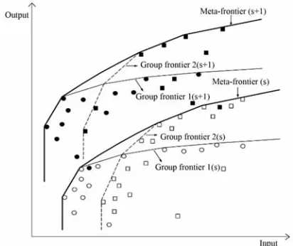
The relation between the group-frontiers and meta- frontiers, the group-productivity change, and meta-pro- ductivity are shown in Figure 1. In Figure 1, we assume that there are only two group-frontiers for the conven- ience of explanation. We can measure group-technical efficiency based on the group frontier for each first time period (s), respectively, and derive the meta-frontier en- veloping the two group frontiers.
Measuring technical efficiency with might differ from measuring it with group frontier. Likewise, the meta- productivity change can be estimated on the basis of the meta-frontier for the two time periods.
Furthermore, general productivity change can be mea- sured on the basis of the group-frontiers between two time periods. The two productivity changes can show which frontiers are farther extended between a group- frontier and a meta-frontier for the two time periods.
3. Data and Empirical Result
In China, the statistical data of inputs and an output are available from the Chinese Statistical Yearbook. We used the data of inputs (labor and capital), an output (added value) of thirty one provinces within three local economies in China during 1995-2008 [35].
[image:5.595.76.288.83.180.2]The capital stock of each province in China was esti- mated by accumulating new investment data through the perpetual inventory method, which is based on the in- vestment of fixed assets from Chinese Statistical Year- book. Here, the initial capital stock was estimated by using new investment for initial certain periods and the average growth rate of initial new investment, as in Young (1995)1. As in existing studies such as Young (1995), we used a depreciation rate of 6 percent.
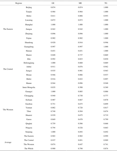
Table 1 shows the group-technical efficiency (GE), the meta-technical efficiency (ME), and the technology gap (TG). When it comes to the group-technical effi- ciency, the average of the whole China is 0.900. Among the three regions, the central region represents the highest level (0.937) while the eastern region is 0.903 and the western region is 0.874, respectively. Taking a closer look at this, in the central region, Heilongjiang shows the maximum efficiency, 1.000 whereas Shanghai shows the
1
The estimation formula according to the perpetual inventory method is as follows:
1 1
K I g
in which K(1) is capital stock in the 1st term, I(1) is new investment in the first term, δ is the depreciation rate, and g is the annual growth rate of new investment in the five initial years. Therefore, constant capital stock is calculated by the following formula:
Table 1. The efficiency and technology gap (1995-2008 year).
Regions GE ME TG
Beijing 0.874 0.874 1.000 Tianjin 0.984 0.984 1.000 Hebei 0.811 0.806 0.993 Liaoning 0.872 0.872 1.000 Shanghai 1.000 1.000 1.000 Jiangsu 0.942 0.942 1.000 Zhejiang 0.896 0.896 1.000
Fujian 0.982 0.982 1.000 Shandong 0.920 0.916 0.996 Guangdong 0.997 0.997 1.000 The Eastern
Hainan 0.651 0.651 1.000 Shanxi 0.848 0.737 0.869 Jilin 0.992 0.823 0.830 Heilongjiang 1.000 0.868 0.869
Anhui 0.911 0.876 0.962 Jiangxi 0.935 0.901 0.963 Henan 0.946 0.886 0.937 Hubei 0.916 0.822 0.897 The Central
Hunan 0.944 0.896 0.948 Inner Mongolia 0.835 0.308 0.369
Guangxi 1.000 0.885 0.886 Chongqing 0.940 0.730 0.777
Sichuan 0.987 0.867 0.878 Guizhou 0.751 0.675 0.899 Yunnan 0.882 0.720 0.817 Tibet 0.748 0.504 0.674 Shaanxi 0.939 0.675 0.719
Gansu 0.849 0.678 0.799 Qinghai 0.759 0.506 0.666 Ningxia 0.794 0.526 0.663 The Western
Xinjiang 1.000 0.692 0.692 The Eastern 0.903 0.902 0.999
The Central 0.937 0.851 0.909 The Western 0.874 0.647 0.741 Average
The Whole 0.900 0.790 0.874
Figure 1. The relation between group-frontiers and meta-frontiers.
maximum efficiency in the eastern region. In the western region, Guangxi and Xinjiang show the maximum effi- ciency. Regarding the meta-technical efficiency, however, the average of the whole China is 0.790, dropping shar- ply compared to the group-technical efficiency. Among the three regions, the eastern region shows the highest level (0.902), while the central region is 0.851 and the western region is 0.647, respectively. As we have seen above, in the eastern region, Shanghai still shows the- maximum efficiency, 1.000, in terms of the meta-fron- tier. Meanwhile, there is no region showing the maxi- mum efficiency in both the other regions. It is interesting that even though Heilongjian, Guanxi, and Xinjiang in the fringe regions are exactly same with the maximum efficiency when it comes to the group-technical effici- ency, the technical efficiency decreased relatively when it comes to the meta-technical efficiency. Therefore, we see that the provinces in the central region are outstan- ding in terms of the relative technical efficiency under the group-frontier, the technical efficiency, however, decreased a lot under the meta-frontier that integrates the entire three regions.
As Table 1 represents, meta-technical efficiency is lower than group-technical efficiency, on average, in the three regions. However, the gap between the group- technical efficiency (0.903) and the meta-technical effi- ciency (0.902) in the eastern is the smallest level among the regions, and then its technology gap (0.999) is almost one (1). The technology gap shows how far the group- frontier is from the meta-frontier; if the technical gap is one (1), it indicates that the two frontiers are the same.
When it comes to the technical gap, while the whole eastern region shows 0.999, the central and western re- gions show 0.909 and 0.741, respectively, indicating that the frontier of the group-technical efficiency in the east- ern region is much closer to the meta-frontier and the
remainder regions are farther away from the me efficien- cies of the provinces in the three regions, almost all provinces in the eastern region have a comparative ad- vantage, while no region shows an advantage in the other regions. We believe the reason most provinces in the eastern outperform those in both other regions is due to various factors, such as developed industrial infrastruc- ture, intensive industrial clusters, sophisticated produc- tion facilities, and strong government support. The well- developed industrial infrastructure has contributed to the eastern region’s significant development combined with adequate transport system. And this advantage has made it easy to access natural and human resources. The clus- ters where resources and competencies have been con- centrated to produce a competitive advantage in a spe- cific industry have been promoted and are predominantly located in the coastal region since the early 1980s. Even though there are some clusters going over other provin- ces, coastal area has become famous for their particular industrial advantages. The eastern area has experienced highly sophisticated production facilities through foreign invest and technical cooperation with foreign partners2. This factor has been also important to improve the rapid development of the eastern region. In addition, the gover- nment has continued to support this region administra- tively and financially. Especially, government expendi- tures on education, public service and R&D, com- pounded with so-called preferential policies, have pro- moted the regional technical efficiency dramatically.
Even though the central region has recently pursued the rapid economic development with a large stock of physical capital, it does not seem to overtake the eastern region which has been advantageously positioned for high-tech industries with a variety benefit from FDIs. In addition, although the provinces in the central region are outstanding in terms of the relative technical efficiency under the group-frontier, the technical efficiency de- creased a lot under the meta-frontier that envelops the entire three regions. Hence, with respect to the group- frontier, it can lead to distorted estimates of efficiency scores. Meanwhile, since the mean efficiency of the western region is particularly low, this area needs not only to facilitate knowledge diffusion within region but also to adopt the advanced technology from other regions, especially from the eastern area in order to improve its efficiency score and reduce technology gap. Economic and technological cooperation and joint development between two regions also need to be strengthened. Moreover, utilizing its own advantages such as abundant
2The eastern region has received the most benefit from FDIs (Foreign
Table 2 shows the productivity change and the pro- uctivity gap of thirty one provinces in the three regions natural endowment and low labor is still important to
contribute to its efficiency. d
Table 2. The meta-productivity and productivity gap (1995-2008 year).
Group-frontier Meta-frontier MPG Regions
MP TC EC MMP TC EC
Beijing 1.025 1.034 0.991 1.025 1.034 0.991 1.000 Tianjin 1.036 1.029 1.008 1.036 1.029 1.008 1.000 Hebei 0.972 0.987 0.985 0.978 0.992 0.986 1.007 Liaoning 1.013 1.027 0.987 1.013 1.027 0.987 1.000 Shanghai 1.063 1.063 1.000 1.063 1.063 1.000 1.000 Jiangsu 1.021 1.031 0.990 1.021 1.031 0.990 1.000 Zhejiang 1.011 1.032 0.981 1.011 1.032 0.981 1.000 Fujian 0.990 1.001 0.989 0.993 1.004 0.989 1.003 Shandong 0.983 0.997 0.986 0.988 1.002 0.986 1.005 Guangdong 1.030 1.028 1.002 1.030 1.028 1.002 1.000 The Eastern
Hainan 1.022 1.018 1.005 1.022 1.018 1.005 1.000 Shanxi 1.030 1.035 0.995 1.001 1.000 1.002 0.972 Jilin 1.068 1.067 1.001 0.996 1.006 0.991 0.933 Heilongjiang 1.052 1.052 1.000 1.014 1.010 1.005 0.964 Anhui 0.953 0.967 0.986 0.951 0.976 0.974 0.998 Jiangxi 0.959 0.981 0.978 0.947 0.981 0.966 0.987 Henan 0.985 0.992 0.993 0.972 0.984 0.989 0.987 Hubei 0.994 1.004 0.990 0.975 0.988 0.988 0.981 The Central
Hunan 0.990 0.989 1.001 0.976 0.984 0.993 0.986 Inner Mongolia 1.136 1.100 1.033 1.081 1.050 1.029 0.951 Guangxi 0.995 0.995 1.000 0.963 0.978 0.985 0.967 Chongqing 1.008 1.020 0.988 0.950 0.987 0.963 0.943 Sichuan 0.993 1.000 0.994 0.946 0.974 0.971 0.952 Guizhou 0.964 0.956 1.009 0.675 0.972 0.989 0.899 Yunnan 1.011 1.021 0.991 0.967 0.985 0.982 0.956 Tibet 1.012 1.012 1.000 0.987 0.996 0.990 0.975 Shaanxi 1.021 1.016 1.005 0.977 0.987 0.991 0.957 Gansu 1.023 1.020 1.003 0.981 0.986 0.995 0.958 Qinghai 1.017 1.008 1.009 1.018 1.023 0.996 1.001 Ningxia 1.011 1.009 1.002 1.007 1.017 0.990 0.996 The Western
Xinjiang 1.040 1.040 1.000 1.013 1.030 0.984 0.975 The Eastern 1.015 1.022 0.993 1.016 1.024 0.993 1.002 The Central 1.003 1.010 0.993 0.979 0.991 0.988 0.976 The Western 1.018 1.016 1.003 0.988 0.999 0.989 0.970 Average
The Whole 1.014 1.017 0.997 0.995 1.005 0.990 0.981
1) TC and EC in this table mean technical change and efficiency change, respectively while MP, MMP and MPG mean Malmquist productivity, meta-Malmquist produc-tivity and Malmquist producproduc-tivity gap, respectively. 2) TC and EC in this table mean technical change and efficiency change, respectively while MP, MMP and MPG mean
in China over the same time period. While the technical efficiency compares the different production units in a single time period, the productivity change represents the shifting level of the productivity in two different time periods. As mentioned earlier, in this analysis, the pro- ductivity growth is derived from four directional distance functions in the two time periods, s and s + 1. Here, we divide the productivities into the group-productivity change by the group-frontier, and the meta-productivity change by the meta-frontier, and the productivity gap between the two productivities.
The annual group-productivity of the whole China shows 1.014 indicating that it has gradually improved at a rate of 1.4 percent on average over the same period. In terms of the group-productivity, the western region shows the highest level among the three regions since the annual productivity of the western is 1.018 while those of the eastern and the central are 1.015 and 1.003, respect- tively. However, the annual meta-productivity of the whole China shows 0.995 indicating that it has gradually declined at a rate of 0.05 percent on average over the same period, dropping sharply compared to the group-productivity. Based on the meta-productivity, the eastern is the only one region to show the productivity improve-ment among the three regions since the eastern region is 1.016 while the central region and the western region are 0.979 and 0.988, respectively. It implies that the eastern region has contributed to the rapid expansion of the fron- tier annually, while in both other regions they havenot. Taking a closer look at each region, almost all provinces in the eastern region showed productivity growth. These are the same provinces in this area with respect to both the group-productivity and meta-productivity as shown by the productivity gap of at least, 1.000, indicating that the group-productivity change in the eastern region is the exactly same with (or higher than) that of the meta-frontier.
In the central region, Jilin, Heilongjiang, and Shanxi represent productivity growth under group-frontier, while the productivity of these provinces drops sharply regard-ing the meta-frontier. Whereas most of the provinces in the western region show productivity growth with respect to group-productivity, the productivity of these provinces is relatively low regarding the meta- productivity. How-ever, several provinces such as Inner Mongolia, Ningxia, Xinjiang, and Qinghai still show the productivity growth, in terms of meta-productivity. The interesting thing is that Inner Mongolia represents the highest level of pro- ductivity among thirty one provinces, even regarding the meta-frontier. We believe that this is because the western region, especially, Inner Mongolia has become a hot in- vestment spot since the Chinese government has invested
huge money on “the Development of Western China”3. As far as MPG is concerned, however, Inner Mongolia shows productivity decline as shown by the Malmquist productivity gap of 0.951. Whereas all provinces in the eastern region represent productivity growth as shown by the Malmquist productivity gap of, at least 1.000, almost all provinces in the western region represent productivity decline despite showing productivity growth with respect to the meta-productivity in half of the region.
As stated above, Malmquist Productivity (MP) index allows us to identify if its productivity change comes from efficiency change or technical change. In other words, we can check whether the productivity change originates from the progress of new technology (techni- cal change) or the utilization of the old technology (effi- ciency change). Table 2 also shows the decompositions of MP and MMP into technical change and efficiency change of the three regions in China, respectively.
With respect to the group-productivity of the whole China is 1.014, decomposed into TC (1.017) and EC (0.997), implying that the productivity growth at the rate of 1.4 percent comes from the technical change rather than the efficiency change. By happenstance, the techni- cal change is a main factor in all three regions. The re- sults of this study are similar to those of Park, et al. (2012) even though they compared productivity per- formances prior to and after China’s 2001 entry into the World Trade Organization (WTO).
On the other hand, the productivity of the whole China is 0.995, decomposed into TC (1.005) and EC (0.990) with respect to the meta-productivity. It means that the productivity decline at the rate of 0.05 percent of the whole China comes from the efficiency change rather than the technical change, regarding the meta-produc-tivity.
In the case of the eastern region, the technical change is a main component to the productivity growth since the technical change (1.024) is higher than the efficiency change (0.993). Meanwhile, it is hard to say that the effi- ciency change is a main factor of the productivity decline in the central area exactly since the efficiency change score is very similar with the technical change score.
3In 2000 China started a develop-the-west campaign. The 10
This is because although the technical change ratio has increased, the efficiency change ratio has decreased in this region as time goes by.
Consequently, regarding the meta-frontier, the produc- tivity declines in the central and western regions have been mainly led by the drop on the efficiency change rather than by the technical change. This might be ex- plained by the fact that the eastern region has received the benefits from utilizing of FDIs, investment of R&D (Research and Development), geographically suitable infrastructures, well-trained and hard-working human capital, and consistent government support since China’s active reform and opening-up. Thus, it suggests that, in order to shrink the gap between the eastern and the other regions, the provinces in central and western regions should pay attention to not only generate capacity for FDIs, R&D and decent infrastructures of transportation and logistics, but also to facilitate an abundant well- trained labor force. In addition, government support avai- lable to business, including advice, financial support, government-sponsored industrial promotion and net- works for innovation and R&D can help make those re- gions more competitive. We also see that there exists a possibility to overestimate of the group-productivities, giving wrong information and distort a reality, especially to policy makers.
4. Conclusions
In this study, we empirically investigated the group- technical efficiencies, the meta-technical efficiencies, and the productivity changes and the meta-productivity changes in thirty one provinces in three regions of China for 1995 through 2008, adopting meta-frontier model. In addition, we decompose the productivity into the techni-cal progress change and technitechni-cal efficiency change in order to examine the determinants of these changes. Here are our findings from this analysis: Firstly, regarding the meta-frontier, the eastern region shows the highest levels in terms of productivity as well as technical efficiency among the three regions. This indicates that the frontier of the technical efficiency and the productivity in the eastern region is closer to the meta-frontier, and the re- mainders are farther away from the meta-frontier, imply- ing that the eastern region has contributed to the rapid expansion of the frontier annually, while in both other regions they have not. Although the provinces in the cen- tral region are outstanding in terms of the relative tech- nical efficiency under the group-frontier, the technical efficiency decreases a lot under the meta-frontier that integrates the entire three regions. Hence, with respect to the group-frontier, it can lead to distorted estimates of efficiency scores. Meanwhile, the mean efficiency of the western region is particularly low. It suggests that this area needs not only to facilitate knowledge diffusion
within region but also to adopt the advanced technology from other regions, especially from the eastern area in order to improve its efficiency score and reduce techno- logy gap. Economic and technological cooperation and joint development between two regions also need to be strengthened.
Secondly, with respect to the meta-productivity change, the productivity declines in the central and western re-gions have been mainly led by the drop on the efficiency change rather than by the technical change while the productivity growth in the eastern region has been led by the technical change. This might be explained by the fact that the eastern region has received the benefits from utilizing of FDIs, investment of R&D, geographically suitable infrastructures, well-trained human capital, and consistent government support since China’s active re- form and opening-up. It suggests that provinces in the central and western regions need to not only generate capacity for FDIs, R&D, and decent infrastructures of transportation and logistics, but also to seek an abundant well-trained labor force. In addition, government support available to business, including advice, financial support, government-sponsored industrial promotion and net- works for innovation and R&D can help make those re- gions more competitive.
Lastly, apart from the general traditional frontier methodology, we apply the meta-frontier to our analysis and find a very important fact that there exists a differ- rence between the group-frontiers and the meta-frontiers by applying the meta-frontier; the meta-frontier is lower than the group-frontier. Since the circumstances include- ing technology, human capital, natural endowment, eco- nomic policies, and government expenditure in each re- gion are quite different to each other, the traditional effi- ciencies (productivities) under different production fron- tiers may not be comparable among these heterogeneous groups. It implies that ignoring the variation across the groups could lead to biased estimates of the production frontier, and thus it could mislead policy implications.
REFERENCES
[1] http://www.worldbank.org/[2] W. Meeusen and J. Van den Broeck, “Efficiency Estima- tion from Cobb-Douglas Production Functions with Com- posed Error,” International Economic Review, Vol. 18, No. 2, 1977, pp. 435-444. doi:10.2307/2525757
[3] D. J. Aigner, C. A. K. Lovell and P. Schmidt, “Formula- tion and Estimation of Stochastic Frontier Production Function Models,” Journal of Econometrics, Vol. 6, No. 1, 1977, pp. 21-37.
doi:10.1016/0304-4076(77)90052-5
Vol. 13, No. 1, 1980, pp. 5-25. doi:10.1016/0304-4076(80)90040-8
[5] J. Jondrow, C. A. K. Lovell, I. S. Materov and P. Schmidt, “On the Estimation of Technical Inefficiency in the Sto- chastic Frontier Production Function Model,” Journal of
Econometrics, Vol. 19, No. 2, 1982, pp. 233-238. doi:10.1016/0304-4076(82)90004-5
[6] S. C. Kumbhakar and C. A. K. Lovell, “Stochastic Fron- tier Analysis,” Cambridge University Press, Cambridge, 2003.
[7] M. M. Pitt and L. F. Lee, “The Measurement and Sources of Technical Inefficiency of Indonesian Weaving Indus- try,” Journal of Development of Economics, Vol. 9, No. 1, 1981, pp. 43-64. doi:10.1016/0304-3878(81)90004-3 [8] C. Cornwell, P. Schmidt and R. C. Sickles, “Production
Frontiers with Coss-Sectional and Time-Series Variation in Efficiency Levels,” Journal of Econometrics, Vol. 46, No. 2, 1990, pp.185-200.
doi:10.1016/0304-4076(90)90054-W
[9] G. E. Battese and T. J. Coelli, “Prediction of Firm-Level Technical Efficiencies with a Generalized Frontier Pro- duction Function and Panel Data,” Journal of Econo-
metircs, Vol. 38, No. 3, 1988, pp. 387-399. doi:10.1016/0304-4076(88)90053-X
[10] S. E. Atkinson and C. Cornwell, “Parametric Measure- ment of Technical and Allocative Inefficiency with Panel Data,” International Economic Review, Vol. 35, No. 1, 1994, pp. 231-244. doi:10.2307/2527099
[11] Y. H. Lee and P. Schmidt, “A Production Frontier Model with Flexible Temporal Variation in Technical Effici- ency,” In: H. Fried, C. A .K. Lovell and S. Schmidt, Eds.,
The Measurement of Prodcutive Efficiency; Techniques
and Applications, Oxford University Press, Oxford, 1993. [12] S. C. Kumbhakar, “Production Frontiers, Panel Data, and
Time-Varying Technical Inefficiency,” Journal of
Eco-nomics, Vol. 46, No. 1-2, 1990, pp. 201-211.
[13] G. E. Battese and T. J. Coelli, “Frontier Production Func- tions, Technical Efficiency and Panel Data: With Appli- cation to Paddy Farmers in India,” Journal of Produc-
tivity Analysis , Vol. 3, No. 1-2, 1992, pp. 153-169. doi:10.1007/BF00158774
[14] A. Charnes, W. Cooper and E. Rhodes, “Measuring the Efficiency of Decision—Making Units,” Journal of Ope-
rational Research, Vol. 2, No. 6, 1978, pp. 429-444. doi:10.1016/0377-2217(78)90138-8
[15] W. D. Cook and Joe Zhu, “Allocation of Shared Costs among Decision Making Units: A DEA Approach,” Com-
puters & Operations Research, Vol. 32, No. 8, 2005, pp. 2171- 2178. doi:10.1016/j.cor.2004.02.007
[16] W. D. Cook and M. Kress, “Characterizing an Equitable Allocation of Shared Costs: A DEA Approach,”
Euro-pean Journal of Operational Research, Vol. 119, No. 3, 1998, pp. 652-661. doi:10.1016/S0377-2217(98)00337-3 [17] L. Friedman and Z. Sinuany-Stern, “Combining Ranking
Scales and Selecting Variables in the DEA Context: The Case of Industrial Branches,” Computers & Operations
Research, Vol. 25. No. 9, 1998, pp. 781-791. doi:10.1016/S0305-0548(97)00102-0
[18] M. Asmild and J. L. Hougaard, “Economic Versus Envi- ronmental Improvement Potentials of Danish Pig Farms,”
Agricultural Economics, Vol. 35, No. 2, 2006, pp. 171- 181. doi:10.1111/j.1574-0862.2006.00150.x
[19] A. Assaf, C. P. Barros and A. Josiassen, “Hotel Effici- ency: A bootstrapped metafrontier approach,” Internatio-
nal Journal of Hospitality Management, Vol. 29, No. 3, 2010, pp. 468-475. doi:10.1016/j.ijhm.2009.10.020 [20] K. H. Chen, Y. J. Huang and C. H. Yang, “Analysis of
Regional Productivity Growth in China: A Generalized Meta-frontier MPI Approach,” China Economic Review, Vol. 20. No. 4, 2009, pp. 777-792.
doi:10.1016/j.chieco.2009.05.003
[21] G. E. Battese and D. S. P. Rao, “Technology Gap, Effi- ciency, and a Stochastic Meta-frontier Function,” Inter-
national Journal of Business and Economics 1, Vol. 1, No. 2, 2002, pp.87-93.
[22] Y. Hayami, “Sources of Agricultural Productivity Gap among Selected Countries,” American Journal of
Agri-cultural Economics, Vol. 51, No. 3, 1969, pp. 564-575. doi:10.2307/1237909
[23] Y. Hayami, “On the Use of the Cobb-Douglas Production Function on the Cross-Section Analysis of Agricultural Production,” American Journal of Agricultural Econom-
ics, Vol. 52, No. 2, 1970, pp. 327-329. doi:10.2307/1237509
[24] Y. Hayami and V. W. Ruttan, “Agricultural Productivity Differences among Countries,” American Economic Re- view, Vol. 60, No. 5, 1970, pp. 895-911.
[25] Y. Huang and V. W. Ruttan, “Agricultural Development: An International Perspective,” Journal of Development
Economics, Vol. 26, No. 1, 1971, pp. 197-200.
[26] M. M. Jemaa and M. A. Dhif., “Agricultural Productivity and Technological Gap between MENA Region and Some European Countries: A Meta-Frontier Approach,”
Economic Research Forum, 2005, pp.1-20.
[27] S. Rungsuriyawiboon and X. B. Wang, “Recent Evidence on Agricultural Efficiency and Productivity in China: A Meta-Frontier Approach,” Discussion Paper No. 104,
Asian-Pacific Productivity Conference, 2007.
[28] C. J. O’Donnell, D. S. P. Rao and G. E. Battese, “Meta- Frontier Frameworks for Study of Firm-Level Efficien-cies and Technology Ratios,” Empirical Economics,Vol. 34, No. 2, 2008, pp. 231-255.
doi:10.1007/s00181-007-0119-4
[29] C.-T. Chen, J.-L. Hu and J.-J. Liao, “Tourists’ Nationali- ties and the Cost Efficiency of International Tourist Ho- tels in Taiwan,” Africa Journal of Business Management, Vol. 4, No. 16, 2010, pp.3440-3446
[30] S.-M. Kang and S.-k. Jo, “Technical efficiency and Tech- nical Gap of Strategic Industries of Busan Using Meta- frontier,” Korean Association of Regional Studies, Vol. 17, 2009, pp.49-73.
[31] K. Denny, C. Harmon and S. Redmond, “Functional Lit- eracy, Educational Attainment and Earnings—Evidence from the International Adult Literacy Survey”, IFS Working Paper W00/09, 2002.
Higher US Wage Inequality?” Review of Economics and
Statistics, Vol. 87, No. 1, 2005, pp.184-193. doi:10.1162/0034653053327649
[33] K. De Witte, W. Groot and H. M. Van den Brink, “The Efficiency of Education in Generating Literacy: A Sto- chastic Frontier Approach,” Review of Economics & Fi-
nance, Vol.2, No. 2, 2012, pp. 25-37.
[34] P. Khrueathai, A. Untong, M. Kaosa-Ard and R. A. Vil- lano, “Measuring Operation Efficiency of Thai Hotels In-
dustry: Evidence from Meta-frontier Analysis,” Journal
of European Economy, Vol. 11, 2012, pp. 202-217. [35] http://www.stats.gov.cn