Strategies for Deeper Integration: Case Study of the Baltics

Munich Personal RePEc Archive

Strategies for Deeper Integration: Case

Study of the Baltics

Lastauskas, Povilas and Biči¯

unait˙e, Audr˙e

Trinity College, Cambridge, Euromonitor International

25 December 2012

Online at

https://mpra.ub.uni-muenchen.de/43321/

Strategies for Deeper Integration: Case Study of the Baltics

ú

Audr˙e Bi i¯

unait˙e

Euromonitor International lnc.

Povilas Lastauskas

University of Cambridge

December 25, 2012

Abstract

When we talk about international integration, trade and investment, the it’s-all-about-geographic-proximity is a tempting argument to make. While the importance of geographic closeness cannot be denied, empirical evidence suggests existence of other, perhaps equally significant factors that bring countries closer together. The aim of this paper is to sketch some light on an often overlooked aspect of international integration, recently introduced as the ‘new regionalism’ paradigm. Based on the proposed ‘mentoring’ and ‘the training ground’ concepts we analyze such integration within the Baltic Sea region, suggesting an alternative approach to international economic convergence.

JEL Classification: F15, F20, C30

Keywords: Mentoring, Economic Integration, Gravity, Baltics

∗_{A more technical version of this paper has been awarded the Olga Radzyner Award for the work on the European Economic}

Integration by the Oesterreichische Nationalbank, Austria. However, all ideas expressed in the paper rest with the authors and shall not be associated with any of the institutions. The usual disclaimer applies.

†_{Address at: Faculty of Economics, University of Cambridge, Sidgwick Avenue, Cambridge, CB3 9DD. Email:}

[email protected], WEB: www.lastauskas.com.

1 Introduction 2

1

Introduction

In the world where modern technology develops at unprecedented rates and mobility levels are greater than ever before one may begin to assume that ties between countries, whether economic or political, are based on conscious and rational decisions to cooperate, rather than physical, financial, cultural, historic, or any other ‘given’ parameters. The idea of the European Union, and especially its expansion to EU27, is largely based on this assumption: being relatively small in territory, Europe posts big verbal and cultural diversity and geographic variation, in addition to diff_{erent country-level interpretations of historic past and massive} disparities between purchasing power and living standards, especially between the “old” Europe and EU newcomers. Still, European integration is believed to be both possible and plausible, and on a number of levels it seems to work.

Looking at Europe more closely, however, one can spot that European integration often starts on a sub-regional level, forming regions within regions, systems within systems. Recently,de Prado Yepes(2007) concluded: “‘New regionalism’ paradigm is a multidimensional form of integration, which includes economic, political, social, and cultural aspects and thus goes far beyond the goal of creating region-based free trade regimes or security alliances of earlier regionalisms”. What constitutes a region, what are the factors that foster regional integration and what it means to participating countries therefore become interesting aspects of the overall international integration topic.

2

Integration of Baltic Sea region: theory and practice

2.1

Costs and gains of region-building

The dictionary gives the following definition of a region: “Region: a relatively large territory, possessing physical and human characteristics that make it a unity distinct from neighbouring regions or within a whole that includes it”. The Baltic Sea region, including Sweden, Denmark, Norway, Finland, Estonia, Latvia and Lithuania, is an interesting mix of political will, pragmatism, and spontaneous economic and cultural forces. Their integration is largely defined by a geographical unity that derives from a common link: the Baltic Sea, but member countries also share a common cultural background, political rationality and even a natural competitive advantage in human communication, merely because of regional linguistic peculiarities. Although the lingua franca of the region is English, some countries share their own common ‘language’. For instance, members of the Nordic cooperation speak so-calledskandinaviska(common Scandinavian) among themselves. Linguistic closeness also adds to easier communication between Finns and Estonians, whereas Russian remains the least complicated international language tool for most Latvians and Lithuanians.

The region has a long history of integration starting with the establishment of the Hanseatic League (Hanse) in the 13th century. This economic alliance was sustained for the following four hundred years, based on similarities such as independent city status and respective locations along key trade routes. Intra-regional progress was interrupted by hostile political forces at the end of the 18th century. For nearly 300 years the Baltic Sea region was split into two rough blocks: the Northwestern, comprised of Sweden, Denmark, Norway and Finland, which developed following Western European market patterns, and the Southeastern, consisting of Estonia, Latvia and Lithuania. These three largely remained under Russian influence: as part of Russian Empire and, from the 20th century onwards, incorporated in the market planning of the Soviet Union.

The relationship between Northwest and Southeast was resumed for a couple of decades in between the two World Wars, when the concept of Nordic-Baltic partnership was remembered by young intellectuals. The idea persisted during the World War II, and the Baltoscandian Confederation by Professor Kazys Pakš_{tas was published in 1942. To this date it is seen as one of the most original publications regarding} the vision of the Baltic Sea region: although a small-scale, but specific study creating grounds for cultural, economic and political cooperation between Baltic and Scandinavian nations. Back in the middle of the 20th century, in the whirl of the World War II, the project came as a challenge that an utopian vision of Northern-European cooperation is possible.

2 Integration of Baltic Sea region: theory and practice 3

the EU is often recognised as the main motivation for this integration, it is in fact a false credit. Sweden, Denmark and Finland all signed free trade agreements with Lithuania, Latvia and Estonia long before they joined the EU, and the level of country-to-country relationship inside the Baltic Sea region remains beyond their links with other EU nations.

The Baltic Sea region was the first multinational region in the world that which set joint goals and action plans to implement sustainable development.1 _{This relatively new idea referred to development that}

met the needs of the present without lowering the ability of future generations to meet their own needs. A central role in the Baltic Sea region was played by the Baltic 21 project, founded as a regional equivalent to the UN Agenda 21, aiming for sustainable development in the Baltic Sea region by serving as a forum for cooperation across borders and between stakeholder groups.

The EU itself has recently acknowledged that such ‘new regionalisation’ - as defined byde Prado Yepes (2007) - may be a logical middle step in creation of the common European market. In 2009, the Baltic Sea region2 _{was officially announced as the EU’s first ‘macro region’, recognising strong economic links and}

tradition. European Union Strategy for the Baltic Sea Region reads: “The Baltic Sea Region is a highly heterogeneous area in economic, environmental and cultural terms, yet the countries concerned share many common resources and demonstrate considerable interdependence. <...> It is a good example of a macro region – an area covering a number of administrative regions but with suffi_{cient issues in common to justify} a single strategic approach.” The Baltic Sea countries, being a part of the EU, quite clearly form a separate region on their own, as illustrated by Table2.1.

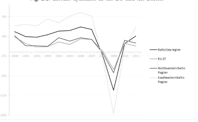
In many dimensions the Baltic Sea region already performs better than the EU27 average. It is par-ticularly strong in public finances, most of education parameters, and demonstrates impressive economic growth and productivity gains over the last decade. Capital flows from the cash-rich Northwest serve as a boost for Southeast economies, off_{ering lucrative returns for investors at the same time. An indirect, but} perhaps an even more desirable eff_{ect is the increased FDI attractiveness of the Baltic Sea region as such.} The sheer market size is one of the strongest determinants of where foreign firms invest, and by harmonising investment climate and increasing political and macroeconomic stability across the region Baltic Sea coun-tries can off_{er prospective investors a larger market, and hence secure greater bargaining power for itself as} a unit. As a result, the entire Baltic Sea region has been way ahead of the EU in terms of real GDP growth since 2000.

Lower than EU performance is in most cases explainable by the typical market structure and growth patterns of newly developing countries; in this case nations from what was previously known as the Eastern Block. The level of GDP per capita is of course lower in the former planned economies of Estonia, Latvia and Lithuania than in Scandinavian countries. Parameters like R&D expenditure and life-long learning indicators are quite naturally inferior in the Southeastern part of the region if compared to Sweden or Finland, but even they are improving rapidly. Public spending on education in the Baltic Sea Region – both Northwest and Southeast – is already considerably higher than the EU average, and so are tertiary enrolment numbers. The entire region is characterised by strong education culture: in 2010, 75% of all high school leavers from around the Baltic Sea continued their education in tertiary institutions, compared to just 61% in the EU.

Compared to EU27, the Baltic Sea region demonstrates much tougher management over public finances and more responsible crediting practices. Recession that hit Europe in 2008-2009 had a severe economic impact within the Baltic Sea region, resulting in double-digit GDP declines, mainly because countries in it refused to foster consumption by getting into more debt. As opposed to most Western European nations that spent billions of euros on economic stimulus packages and industry bailouts, Baltic and Scandinavian countries allowed for the consumption to drop. Especially the Southeastern states had a very diffi_cult belt-tightening year in both public and private sector, but sustainability of fiscal policies was to be maintained at any cost. Then again, painful austerity measures in 2008-2009 allowed for the region to recover faster than the rest of the EU in 2010 onwards. In 2011, GDP grew 1.5% in EU27, while the Baltic Sea region demonstrated a 4% increase.

Even in the aftermath of the 2009 recession, the region’s central government debt is under control and

1_{Five Years of Regional Progress towards Sustainable Development, Baltic 21 Series No. 1/200.}

2_{The newly presented strategy involves eight EU Member States (Denmark, Estonia, Finland, Latvia, Lithuania, Poland,}

2

In

te

g

ra

tio

n

o

f

B

a

lt

ic

Se

a

re

g

io

n

:

th

eo

ry

a

n

d

p

ra

ct

ic

e

4

Tab. 2.1: Comparison of key development indicators in Baltic Sea region and EU, 2003-2010

Baltic Sea EU27 Northwestern Southeastern Region Baltic Region Baltic Region 2000 2005 2010 2000 2005 2010 2000 2005 2010 2000 2005 2010

Economy

GDP growth (annual %) 5.2 5.5 2.2 3.9 1.9 2.2 4.1 2.8 3.0 6.6 9.1 1.1 Productivity 1.0 8.6 2.5 -8.2 2.3 -0.8 -3.3 5.4 5.3 6.8 13.0 -1.2 Gross savings (% of GNI) 23.9 25.4 24.3 20.4 20.3 18.5 27.9 28.2 25.6 18.6 21.6 22.6

Finance

Central government debt (% of GDP) 36.1 30.7 36.9 57.5 49.0 58.8 50.0 42.4 39.1 8.2 15.2 34.0 Bank liquid reserves to assets ratio (%) 6.9 5.1 5.1 2.3 2.2 2.6 3.0 3.0 2.7 14.8 7.2 7.5 Domestic credit provided by banking

55.7 97.4 118.6 116.3 129.3 160.0 79.3 114.1 152.8 24.3 61.1 84.4 sector (% of GDP)

Education

Public spending on education

14.2 14.5 13.6 11.0 11.5 11.5 14.0 14.4 14.0 14.6 14.6 12.8 (% of government expenditure) (2009) (2009) (2009) (2009) Tertiary enrollment (% gross) 62.7 78.8 75.2 49.7 58.6 61.4 69.0 83.2 80.6 54.3 72.8 67.0 Life-long learning (% of 25-64

13.5 15.0 16.8 7.1 9.6 9.1 18.0 21.3 24.5 4.7 6.6 6.6 population in education or training)

Health

Newborn mortality rate

8.7 6.6 5.0 7.6 6.2 5.1 4.7 4.1 3.3 14.0 10.1 7.2 (per 1,000 live births)

Number of healthy years 58

58.0 62.0 63 61.0 62.0 61 62.0 65.0 52 53.0 58.0

(at birth) (2004) (2004) (2004) (2004)

Technology and legal environment

Internet users (per 100 people) 27.2 66.8 81.1 20.6 51.0 70.8 37.2 81.0 89.7 13.8 47.9 69.5 Start-up procedures to register 5 4.9 4.4 7.4 7.4 5.8 4 3.8 3.8 6.3 6.3 5.3

a business (number) (2003) (2003) (2003) (2003)

3 Mentorship in Baltic Sea region: theory and evidence 5

Fig. 2.1: Income dynamics in the EU and the Baltics

bank liquid reserves to assets ratio is considerably higher here if compared to other EU banks. Yes, public borrowing has been growing in Estonia, Latvia and Lithuania, but it has never come close to numbers seen in EU27, or even in other individual post-soviet countries like Hungary or Poland. Nor have they exceeded those recorded in Scandinavian economies, suggesting some sort of intra-regional understanding of what is sustainable and what is not. But the most interesting aspect here – which is also largely the point of this paper – is that the Baltic Sea region is growing closer together. Our research suggests that the key reason behind that is the ‘training ground’ eff_{ect, which is arguably the most e}ff_{ective form of} integration. The ‘training ground’ concept basically means that well-established Northwestern countries have been helping their developing Southeastern neighbours enter the global marketplace by sharing their experience in education, governance and capacity building, in addition to tackling environmental issues, science and technology, trade and investment and other fields that are regarded as especially conducive for region-building. The Scandinavian-Baltic relationship does not end there. For the past two decades, general ‘training’ within the Baltic Sea region has been supplemented with country-to-country mentoring, which suggests the whole new research angle on integration matters.

3

Mentorship in Baltic Sea region: theory and evidence

Quantifyable links between economies manifest through movements of capital, goods and services, and labour. Together with technological transfer, these are the key ingredients in explaining economic devel-opment. Abstracting from more structural techniques (see Pesaran et al., 2004, or Pesaran and Smith, 2006), we pursue less ambitious but more flexible approach suitable for transition economies. We ground our econometric framework on several theories to justify the reduced form system of economic interdepen-dencies.

Trade can concern factor inputs like capital (FDI) or labour (migration), or goods (pure trade). Thus, by trading goods, a country implicitly exports labour and capital, Vanek (1968). This interdependence suggests the necessity to model all major factor movements together, but this is rarely done in practice (though Bergstrand and Egger (2010) have recently analysed FDI and trade of final and intermediate goods). The reasons for FDI and trade concern not only the proximity-concentration tradeoff_{. Neary} (2009) rationalises the export platform gain to serve third countries whereasRobb and Vettas (2003) link countries’ dominanance in trade and FDI through demand uncertainty and irreversibility of FDI.Javorcik (2004) proves that firms with foreign capital tend to be more productive in Lithuania than firms of entirely domestic ownership.

3 Mentorship in Baltic Sea region: theory and evidence 6

(2006) emphasise complementarity and substitution eff_{ects: higher human capital prevents migration if} wages positively and suffi_{ciently reacts to the increased human capital. Generally, domestic population} (and market size) influence FDI flows into transition economies, Neuhaus (2006). We try to combine the extensive literature on factor movements and macroeconomic dynamics to build a unified model.

3.1

Conceptual Model

Surprisingly little has been done on combining the trade, labour, and investment flows in a systematic way. We mainly draw fromBeine et al.(2001),Galor and Moav(2004) andD’Agosto et al.(2006) to guide our empirical enquiry. The simplest way to think about dynamics is by introducing two-period lived agents, and discrete time that runs to infinity. Individuals decide in the first period whether to invest in human capital and in the second period whether to supply it in the domestic labour market or to migrate. Individuals make decisions sequentially, firstly making action and later ‘picking fruit’. The argument of bequests, which allows mimicking behaviour of an economy peopled by infinite-lived individual agents, explicitly acknowledges the temporal nature of economic integration and maps to empirical exercise.

We will not delve into the details of the infinitely-lived agents in the overlapping generations (OLG) framework. The interested reader is referred to Blanchard and Fisher (1989, Chapter 3). Just note that a time series of agents’ decisions require an introduction of gifts and bequests. The consumption

c times price p (expenditure) must equal the budget constraints which include wages wt, investment

in human capital et, gifts gt made by a youngster to the parents in period t, and bequests bt.

For-mally, q_i´

Ê∈_Ωic1ijt(Ê)pijt(Ê)dÊ = (1≠ut)wt+bt≠gt≠e

i

t © y1jt, where yjt is the net income

af-ter paying for parents, investing in education, and receiving the bequest. The expected income in the second period given the decision in the first period includes the probability to migrate from the region

j, fi1j and the probability (uniform over generations with different human capitals) uj,t+1 to loose the

job in the region j in the period t + 1, also the wage abroad wı

t, the migration cost ·M, the

mea-sure of ability a1, and the measure of human capital h1jt. The basket of goods in the second period is

q

i

´

Ê∈_Ωic2ijt(Ê)pijt(Ê)dÊ=Et−1Wt≠(1 +n)bt+ (1 +n)gt©y2jt.

One can think that at time t, the first generation consumes the basket of goods c1jt, defined over a

continuum of varietiesÊiœΩi, whereidenotes the region and includes all traded and domestically produced

brands, orU1jt=qi

´

Ê∈Ωic1ijt(Ê)

(◊−1)/◊

dÊ (that is, propensity to migrate, work or invest are subsumed to the desire to maximise consumption). The mass of varieties produced in region k is denoted as mk.

Aggregate consumption in the regionjis the sum of consumption by the young and the old agents in period

t: Cjt = (1≠ut)Ltc1jt+ (1≠ut) (1≠fi1jt)Lt−1c2jt, where (1≠fi1jt)Lt−1 is the remaining labour force

after emigration. We assume that all consumers have identical preferences over a continuum of horizontally diff_{erentiated product varieties. Thus, consumption level is solely determined by the income, and not by} attributes such as demographic characteristics.

3.1.1 Migration and human capital

Besides investment to education, another agent’s choice is that of migration, closely related to the com-position of wage. We assume that the wage level is a positive function of the level of human capital. For extremely small and open countries, labour is mostly a function of foreign demand. The probability of unemployment3 _{is equal tou}

t, and it depends on economic conditions of foreign partners. We assume that

Eut+1=E(ut+‘t+1) =ut.We do not analyse unemployment insurance and allow the bequests to act as a

partial insurance.

Then, we have two strands of migrants - those who leave their home for working abroad, and those who attain education at home and then choose whether to migrate or stay at home. If the first dynasty of time t decides to invest e1t in education, it will be able to offer a higher human capital level in the

second period: h2,t+1 =h1t

Ë

1 +a1e—1t

È

where h1tis the human capital of dynasty 1 at timet anda1 is a

parameter of ability uniformly distributed among dynasties on the probability space[a,¯a],and0<—<1. Then, in the second period, the skilled agent’s wage will grow in proportion of additional human capital:

wt+1=wt

1

1 +“1h1t

Ë

a1e—1t

È2

=wt(1 +“1—ht+1), where“1is the expected sensitivity of wages to human

3 Mentorship in Baltic Sea region: theory and evidence 7

capital as well as a condition of labour market in general, and·M is the fixed costs of migration. Presence of fixed costs will generate a threshold level of ability and will partition the ability space, see Supplementary Material (SM). The present value of the lifetime income is discounted by the discount rate rt, which is

equal to the world interest rate at time t.4 _{Hence, the present value of lifetime earnings equals N P V}

t =

(1≠ut)wt−e1t+E((1≠ut+1)wt+1)/(1 +rt) = (1≠ut) [wt+E(wt+1)/(1 +rt)]≠e1t.5Individuals

con-sider investing in human capital if the benefits outweigh costs,wt+1−wt> e1t, or wt > e1t/“1h1t

Ë

a1e—1t

È

provided “1h1t

Ë

a1e—1t

È

> 0. Similarly, the educated migrate if costs are outweighed by the benefits,

wı

t+1≠(1≠ut+1)wt+1>·M, or

wı

t ≠wt+ (wıt“2≠wt“1)h1t

Ë

a1e—1t

È

+ut+1wt+1>·M (3.1)

using wı

t+1 =wıt

1

1 +“2h1t

Ë

a1e—1t

È2

. Therefore, wage diff_{erentials and lost wages due to unemployment} are important factors of migration decisions, both for unskilled and skilled workers.

3.1.2 Trade

Not only agents, but also firms have decisions to make. Firms can produce domestically, engage in trade or capital investment. Note that we are dealing with monopolistically competitive firms. Due to a symmetry, there is a one-to-one correspondence between varieties and firmsmkin regionk. Then, the aggregate inverse

demand functions for each variety are generated from the CES preferences:

pijt(Ê) =C

−1

◊

ijt Yj/

A ÿ

k

mkC

◊−1

◊

kjt

B

, (3.2)

whereCijtis aggregate demand in regionj- variety produced in regioniat timet; andYjt©(1≠ujt) (1≠fi1jt)Ljtyjt

stands for the aggregate income which is available for consumption in regionj at time t. Note that unem-ployed and those who left the country do not earn.

Production ofc units of output requirestc+F units of inputs, wheretis marginal andF is fixed input requirement. Technology is essentially a function of aggregate labour and capital, all expressed in price of labour. Shipping varieties both within and across regions is costly. We model trade cost using the ‘iceberg’ argument, well-known in economic geography when shipping one unit of any variety requires to dispatch ·jkt>1. The value of trade flows from ito j is given byXijt ©mipijtCijt. Combine with price equation

(3.2) and eliminate firm measure to obtain a usual gravity equation:

Xijt=

C◊−

1

◊

ijt

q

k pi

pkYkC

◊−1

◊

kjt

YiYj. (3.3)

The trade costs are calculated using the following expression: log·ij = Îlogdij, where dij denotes the

distance between regionsi andj. Finally, the gravity equation (3.3) can be cast in matrix form where all variables are in logarithms:

X_=—01_+—1Y_{destination+—2}YÂ_origin+—3dÂ_+—4w_{Â +—5}WX_{, (3.4)}

whereW_{= [}S_diag(L_)]¢I_n,1_{is the vector of ones, diag(}L₎

n×n=diag(Li/L)i=1,..., n,all variables with a

tilde are equal toXÂ ©(I≠W₎X_{.They are measured as the deviation from the labour force (L) weighted}

average. Yet, trade is not the only source of interdependence, and we turn to capital now.

4_{As demonstrated by the current financial turmoil, the small open economies may face large liquidity constraints due to}

global risk shocks. In empirical part we therefore employ different interest rates, capturing both accessability of capital and its ‘representative’ pricer_t.

3 Mentorship in Baltic Sea region: theory and evidence 8

3.1.3 Foreign capital inflows

Now we assume that FDI can bring new inputs to an economy thereby promoting competition in domestic input markets. We follow the framework of Razin and Sadka (2001). An increase in input varieties is interpreted as the technology transfer. The production function of varieties isCt=F

1

Kt

1

htLÂt

22

. Capital

is assumed to be a composite good consisting ofN inputs(k1, k2, . . . , kN), Kt =1qN_j=1kj,tÍ

21/Í , where 0<Í<1.Productivity gains arise due to change in the rate of return, which derives via the use of foreign savings to augment the domestic capital stock, technology transfer through increased variety of capital inputs, and the increase in competition in the input market.

Let the available labour stock of the regionjbe used only for the production of intermediate and denote it byL˜jt= (1≠ujt) (1≠fi1jt)Ljt. The number of employees is equal to the ‘endowment’ of the working-age

population Lj0, which is assumed to stay constant across each period minus the migrants outflow EMt,

plus the return migrantsIMt,

(1≠fi1jt)Ljt=Lj0+net migrationt. (3.5)

The net migration (IMt≠EMt) is assumed to depend on future prospects of wage differences, following the

empirical finding that transition economies react to slumps heavily and suddenly, while wages in advanced economies change sluggishly, especially downwards. Hence, any crisis makes migration more attractive. If we keep inputs constant, then output will be increasing in the number of varieties. Hence, trade in intermediate goods generates a form of international increasing returns, see alsoChakraborty(2003).

All producers will serve a diff_{erent variety due to fixed costs. Hence, production of representativekj} requiresak units of overhead capital, constituting the fixed cost: aktrt=Ft, wherertis the rental rate and

Ftis the fixed cost. From before, the marginal cost component isaLt

1

hit

Ë

aie—it

È2

wtwhere the first term is

marginal labour requirement that is smaller for higher level of human capital, and the wage ratewt which

is positively related to the human capital. Finally, each producer will equate marginal costs to marginal revenues which leads to pricepK

it =aLt

1

hit

Ë

aie—it

È2

wt/Í. FDI inflows imply that a firm located in country

j maximizes its profit, given byq_k!pjk≠tpjK·jk"Cjk≠F pKj , thereby yielding the price set by the firms:

pjk =◊/(◊≠1)·jktpKj . The same argument of the zero profit yields the condition that operating surplus

must be of the same magnitude as fixed cost q_kpjkCjk/◊ = F pKj , implying

q

k·jkCjk = (◊≠1)F/t.

Finally, the region-wide resource constraint tells that with the present capital endowment, the lacking capital is brought only from abroad. From the discussion on trade, we hadmipijC¯=Yi·ij,so that

mipiF

1

Kt

1

htLÂt

22

=Yi . (3.6)

Hence, FDI is positively related to the need of capital, given the labour stock. In other words, decreasing labour supply due to emigration requires more FDI to counteract labour movements. Implicitly, wages also determine the need for FDI: the higher the wages, the less capital is needed to satisfy demand. However, the more productive is a worker compared to the cost of education,6 _{the higher is the demand for capital}

from the final goods producers. This explanation does not confront with that of D’Agosto et al. (2006) which claim that FDI increases bilateral information and knowledge on employment, wages abroad, and practices, technical and organizational procedures in foreign enterprises. Neither does it demur toFederici and Giannetti (2008) which claim that migration flows reveal cultural characteristics and labour force features that may stimulate inflows of capital to the emigrants’ homelands.

3.1.4 Linkages between FDI and trade

However, firms can also opt for pure trading instead of investing (FDI). FollowingNeary(2009) operating profits of serving the parent-country market may be expressed as a function of marginal factor costs and

6_{In our framework, investment in education reduces consumption of final goods in the current period, and therefore has a}

4 Empirical Results 9

market access costs. If the multinational remains a domestic firm and supplies home market from its parent facitilies, wherewı

t is the local wage rate, its profits will equalfitı

!

pıK_(wı

t),·

"

.7 _{Alternatively, it can invest}

in the host country, exporting all its output back to the source country and incure a trade cost of·ı

t. The

firm incurs a plant-specific fixed cost fi, and earns operating profits of fiıt

!

pK_(w

t) +·tı,·

"

, where wt is

the host-country wage. Then, the relative profitability of FDI can be captured by the diff_{erence in profits.} Presumably, Baltics possess smaller trade cost than outsiders, which introduces an additional gain from serving the partner-country market, namely the export-platform gain.

Indeed, often overlooked reason for engaging in FDI is preparation for penetrating a large market (Rus-sia), by exploiting small buff_{er-countries which are more West-oriented, predictable and associated with the} target through various linkages. These include widespread knowledge of Russian language, old links between companies and interactions at both commercial and personal levels inherited from the Soviet times. Hence, multinationals may first settle in a less risky environment to explore possibilities of the Russian market, thus making the Baltics their export platforms.

Note that unlikeHead and Mayer(2004), which consider the potential market location, we introduce a new dimension into the analysis. Russia is of suffi_{cient size for engaging in FDI (which has a good growth} potential, too), but the major obstacle is uncertainty, mainly due to political situation. UnlikeRobb and Vettas(2003), which assume that demand uncertainty and irreversibility of FDI give rise to both exports and investment, our argument is thatthe major source of uncertainty is rooted in local knowledge of business practices and links with the ‘right’ authorities in Russia. Hence, the parameter of new capital varietiesnis given by

n=f!·, gtRussia−4 , fi

"

. (3.7)

which decreases the price of capital and increases its productivity. The capital varieties are related to both trade costs and the lagged growth of Russian market, the latter reflecting the time for making a decision. This lays down the foundations for the empirical enquiry.

4

Empirical Results

All region economies must be considered together, as economic integration requires multiple correlations between the region’s constituents. In the empirical exercise, we employed the following variables for the whole Baltic region: MIG _{which denotes a flow of migrants,} w _{is the real log wage,} Y

·is the real log GDP, either destination or origin,r_{is the interest rate vector,}HC_and SoE_{stand for human capital and}

spending on education, d _{is a measure of distances between capital cities (in km),} WX _{is the weighted}

trade flows whereW_{= [}S_diag(L_)]¢I_n, ¢denotes the Kronecker product,S_{is the n}◊_n matrix of ones, diag(L₎

n×n = diag(Li/L)i=1,..., n, where L is the labour force. Then, gRussiat−4 is growth rate of the real

Russian GDP with 4 quarters lag. Finally, we include the set of indicator variables qCs where Cs =1

if s = i, j for the flow between i and j, and zero otherwise. We account for fixed-eff_{ect terms in all} flow equations to control for the general-equilibrium eff_{ects (“multilateral resistance” terms)}8 _{and capture} heterogeneity as suggested byFeenstra (2004) (also seeAnderson and Yotov(2012) which document that fixed eff_{ects are well in line with structural gravity forces). Our setting allows for spatial correlation in the} trade equation which captures interdependence and “hubness” eff_{ect (directing export activities towards} “hub” countries), seeMorales et al.(2011).

The previous discussion points to the estimating system. Therefore, we are dealing with the following relations:

MIG_=”01_+”1w_{Â +”2}Y_{destination+”3}r_+”4HCˆ _+”5SoEˆ ₊q_µMIG_{s Cs+}u_{M IG} X_=—01_+—1Y_{destination+—2}YÂ_origin+—3Âd_+—4w_{Â +—5}WX₊q_µX_sCs+u_X FDI_=Ÿ01_+Ÿ1ÎÂd_+Ÿ2gRussia_{t−4 +Ÿ4}w_Â+Ÿ5MIG_t−4+Ÿ6X_t−4+q_µFDI_{s Cs+}u_{F DI}

(4.1)

7_{Fixed costs are independent of how the firm serves the foreign market, so we followNeary(2009) and omit them.} 8_{The area of estimating gravity is flourishing: early contributions byAnderson(1979) andBergstrand(1985) missed the}

4 Empirical Results 10

where wage equation is estimated to extract relevant information and foreign variation, human capital, and education spending, so that it could be treated as weakly exogenous. The same applies to origin GDP.

Rationalisation of the first equation stems from equation (3.5) combined with migration probability, unemployment, interest rate, stock of human capital and expenses on education enter the equation in levels. Recall that migration probability depends on wages whereas unemployment on trading partners’ income, both variables measured in a deviation form. Trade flows are measured as have been shown in (3.3) and (3.4). Finally, FDI equation is written from (3.6) using the described capital aggregation. Trade costs enter as they have been defined in the trade equation, changes in Russian economic performance as in (3.7), dummies control for system-wide eff_{ects and the cost of entering the market (gains from FDI). Wages enter} the equation because of the FDI gain argument. Trade flows capture the amount of imported goods that can be used for capital formation, and may be one of the channels to introduce capital varieties as in the aggregate capital Kt. Finally, capital production in our model requires labour which is assumed to vary

because of net migration; the local wage depends on human capital stock and investment in education, see the price equations with FDI and constraint in (3.6).

4.1

Data Analysis

We have chosen three Baltic States and their most influential neighbours in terms of trade, migration and FDI. Hence, we consider Scandinavian nations (Finland, Sweden, Norway, and Denmark), Germany and the UK, and Russia. They account for a considerable share of economic activities in the Baltics: usually over 50% of their total linkages with the world. As such, we can reasonably expect that our analysis reflects the most significant relations with the foreign countries. Our data encompass a period from 1992Q1 to 2009Q2, or 70 quarters.9 _{More details on data are provided in SM.}

We started with the unit-root testing, employing the Augmented Dickey-Fuller (ADF) test known for its good power characteristics compared to other unit roots tests. All variables are stationary with migration causing doubts: it demonstrates some outbursts (EU enlargement) but has no clear trend. We report test results without a trend, unless it is clear that a variable is trending (e.g. GDP). This does not, however, aff_{ect conclusions because trend did not change the outcome. Therefore, all variables as they appear in the} system may be treated as stationary; the null of a unit root has been rejected.

9_{The choice of time dimension is dictated by two reasons: first, we wanted to comply with data availability in the early}

4 Empirical Results 11

Tab. 4.1: Unit root tests for the variables in levels

Variable Test Statistic Critical Value Variable Test Statistic Critical Value

logRGDP

DF=-5.0809 ADF(1)=-5.1754 ADF(2)=-5.3422 ADF(3)=-5.4306 ADF(4)=−4.4027

-3.4179 logTrade

DF=-4.1002 ADF(1)=−4.0641

ADF(2)=−4.1234

ADF(3)=−4.2002

ADF(4)=−3.5065

-2.8657

r

DF=-9.9424 ADF(1)=-10.5226 ADF(2)=−11.9337

ADF(3)=−8.5933

ADF(4)=−8.6337

-2.8657 WX

DF= 3.8150

ADF(1)=-3.5572 ADF(2)=−3.6050

ADF(3)=−3.6976

ADF(4)=−3.7066

-2.8657

logHumCap

DF=−5.7245

ADF(1)=-5.8386 ADF(2)=−5.9603

ADF(3)=−6.0903

ADF(4)=−6.1441

-3.4179 logFDI

DF=-13.2361 ADF(1)=−8.9244

ADF(2)=−6.7722

ADF(3)=−5.7589

ADF(4)=−5.4524

-2.8657

logMIG

DF= 3.1883

ADF(1)=−3.2126

ADF(2)=−3.2376

ADF(3)=-3.2632 ADF(4)=3.3030

-2.8657 Russian growth

DF=-22.3056 ADF(1)=−23.6832

ADF(2)=−15.0440

ADF(3)=−10.3806

ADF(4)=−10.6078

-2.8657

logSoE

DF=−9.2347

ADF(1)=-9.7823 ADF(2)=-10.4424 ADF(3)= 11.2595

ADF(4)=−7.9948

-2.8657

Critical values are 95% for the ADF

Since there was no nonstationarity detected, we can turn to the estimation framework that suits our type of data and model.

4.2

Empirical Evidences

We continue with the technique known as seeemingly unrelated regresssion equations (SURE), originally analysed by Zellner (1962). We can treat the system of equations as the restricted multivariate VAR. Moreover, this method allows us to account for direct and indirect eff_{ects between FDI, migration and} international trade.10 _{The latter relationship comes through correlation in errors accross equations. The}

direct eff_{ect is incorporated in equations with the lagged variables of interest. Further, we partially control} for spatial interdependence and account for flows to other countries insofar as they relate to the Baltics. This reveals how Baltic nations aff_{ect each other while dealing with the same partners.}11 _{Results are presented} in Table4.2.

To reassure our choice of SURE, we calculated the Likelihood Ratio (LR) statistics to test whether a non-diagonal error covariance matrix is characteristic to the model. For brevity, we consider Lithuania’s statistic only. The comparison between system log-likelihood to the log-likelihood values for each equation leads toLR=222.2 which is asymptotically distributed Chi-Square with 3 df. The 95 per cent critical value is‰2(3) = 7.81. We strongly reject the hypothesis that the error covariance matrix of the three equations is diagonal, which supports the use of SURE. The same conclusion manifests for Latvian and Estonian systems.

4.2.1 Endogeneity issues

From the system of equations, we can foresee a problem that wage is not unconditionally exogenous variable. Given weak exogeneity, however, implies that estimating conditional distribution parameters is no less effi_{cient than estimation of the full set of parameters of the joint distribution (Greene,2003). Since we are} dealing with the theory implied relations, it is obvious that the wage is influenced by the agents’s decisions, and decisions may be influenced by the wage level (or its diff_{erence between home and foreign levels). The} solution of endogeneity involves the logics of Two-Stage Least Squares (TSLS), proposed byTheil(1953).

10_{It also allows for heteroskedasticity in the generalized SURE, seeBartels and Feibig(1992).}

4

E

m

p

ir

ic

a

l

R

esu

lt

s

1

2

Tab. 4.2: SURE regressions for the Baltic States

Latvia Estonia Lithuania

Variables log MIG log Trade log FDI log MIG log Trade log FDI log MIG log Trade log FDI

Â

w -.10 (.08) .34 (.17)** -.90 (.30)*** -.34 (.11)*** .21 (.17) .98 (.26)*** -.06 (.09) .43 (.15)*** 1.61 (.17)*** Ydest .10 (.03)*** .82 (.04)*** - .17 (.03)*** .42 (.05)*** - .01 (.03) .34 (.04)***

-r .009(.002)*** - - -.007 (.002)*** - - .01 (.002)*** -

-ˆ

HC 1.14 (.06)*** .07 (.10) 1.46 (.07)***

ˆ

SoE -10.12 (.93)*** -7.72 (.87)*** -43.27 (4.74)***

Â

Yorig - 2.15 (.27)*** - - .80 (.07)*** - - .65 (.09)***

-Â

d - -0.55 (1.16) - - .05 (.50) - - .93 (.49)

-WX - .65 (.18)*** - - .31 (.18)* - - .64 (.18)***

-gtRussia−4 - - 7.48 (1.13)*** - - -.31 (1.13) - - .03 (1.21)

MIGt−4 - - .83 (.09)*** - - .12 (.08) - - .82 (.09)***

Xt−4 - - .18 (05)*** - - .23 (.05)*** - - .23 (.05)***

¯

R2=.84 R¯2=.91 R¯2=.22 R¯2=.77 R¯2=.89 R¯2=.31 R¯2=.82 R¯2=.90 R¯2=.27

Note: Number of observations: 770, used in regression: 766 (due to the lagged variables). Standard errors in parentheses. *, **, *** denote significance at 10%, 5% and 1% respectively.

4 Empirical Results 13

Tab. 4.3: Regression results for Latvia

Equation Human capital (HC), Spending on education (SoE), Real wage ,R¯ 2

=.38

¯ R2

=.42 R¯2

=.37 R¯2

=.38

r -.007 (.001)*** .37E-3 (.9E-4)***

-rt−4 - .35E-3 (.9E-4)***

-dummyMIG -.271 (.08)*** .009 (.005)

-logwdestination .29 (.016)*** .013 (.001)***

-logwdestination, t−4 -.1 (.016)*** -.02 (.001)***

-Fitted HC - - .26 (.01)***

Fitted SoE - - -1.5 (.25)***

logYdestination - - .03 (.0065)***

logYdestination, t−4 - - -.02 (.0065)***

Note: Number of observations: 770, used in regression: 766 (due to the lagged variables). Standard errors in parentheses. *, **, ***

denote significance at 10%, 5% and 1% respectively. All specifications include a constant term.

For each Baltic State we estimate equation on human capital which, according to theory, is dependent upon spending on education, interest rates, migration costs and wages abroad. Spending on education may also depend on the quality of human capital, as better educated people tend to invest more in education, especially where future welfare of their children is concerned. As an illustration, refer to Table4.3.

Since we used lagged exogenous variables, autocorrelated error terms may be suspected. Assuming that disturbances follow a stationary autoregressive process with stochastic initial values, a specification with AR errors have been conducted. This procedure is warranted since we do not employ any lagged dependent variables. However, the log-likelihood ratio statistics reveals that the null which postulates AR(1) against standard OLS has been strongly rejected (‰2_{(1) = 1266and‰}2_{(1) = 734for human capital and spending,}

respectively. Human capital equation, however, favoured AR(2) against AR(1), with‰2(1) = 1.18. This was not a case for spending equation where we rejected AR(2) in favour of AR(1) with‰2(1) = 8.4To learn if there is indeed AR(2) error process in the equation of human capital, we performed Cochrane-Orcutt test with the specified lags of AR process, and there were no signals of significant autoregressive behaviour with AR(2) errors (thet≠_{ratio was}≠_{.63). Therefore, we opted for the OLS specification. Then, the fitted values} have been used to estimate the wage equation, see Table4.3.

Another source of endogeneity is the deviation of Baltic countries’ GDPs from the weighted average of partner countries’ GDPs,YÂ_{origin. Its first term, namely domestic GDP, is endogenous because it depends}

on FDI and trade (these components are used in calculating GDP), although trade is also claimed to depend on GDP. Hence, we again employ the same reasoning and regress local GDPs on all exogenous variables, extract exogenous variation, and use fitted values to constructYÂ_origin.

4.3

Interpretation

Estimates after adjustments for endogeneity are reasonably precise as depicted in Table4.2. As expected, adjusted wages negatively aff_{ect migration whereas higher earning potential abroad attracts more Baltic} people. Human capital tends to be positively related to migration flows whereas spending on education is consistently negative and significant. As theory hints, human capital can only be a deterrent of migration if wages react strongly enough to it. Also, education spending reduces current consumption and requires larger future gains, financial in particular. Since receiving countries are human capital abundant, an average migrant may be relatively low skilled (high wage diff_{erential rationalises this, see SM). Then lower investment} is related to more labour outflows. As such, inequality in the Baltics compared to Sweden or the UK may explain why it is particularly “profitable” for low-ability agents to migrate to these countries, which not only have higher average wage, but are also characterised with more equal income distribution.

5 Institutional alliances and ‘training ground’ effect 14

where human capital is not a significant determinant of migration. Trade positively reacts to higher income of partner-countries, as well as origin income level. Intra-regional trade growth has a positive eff_{ect on} smaller Baltic economies (as captured by WX_{). Wage terms are positive which may be rationalised by}

changing demand structure: the smaller the diff_{erence between wages, the higher the trade.}

All Baltic States indeed trade very extensively with their Scandinavian neighbours, as these off_{er good} training ground before entering other Western markets. Meanwhile, FDI has been flowing to Latvia owing to lower wages. This was not a case for Estonia and Lithuania, presumably because higher wages have been associated with higher productivity that outweighed increased costs. Economic development of Russia aff_{ects Latvian FDI significantly and positively; we note that Latvia has the largest Russian diaspora among} the three countries. Moreover, more annual FDI is attracted when trade and migration increased in the previous year year, as more capital is then needed to counteract labour movements. It echoes the results of Javorcik et al.(2011) on FDI and migrants’ flows, especially those of higher education, andCoughlin and Wall(2011) on the eff_{ect of information networks and intensity of trade. This again reassures our unified} treatment of capital, labour and trade flows.

In contrast to gravity literature (see McCallum (1995) which introduced very large negative foreign country eff_{ects for cross-border trading) and despite common sense as regards transportation costs, distance} is a relatively unimportant variable in our findings. Distance does not appear on the list of statistically significant variables, confirming our initial idea that proximity is not the most important factor, especially within well defined regions.12 _{In part, distance-inspired trade costs are outweighed by higher demand and}

presumably better prices in destination countries. More importantly, distance may proxy for deeper factors such as historical, cultural and other qualitative links, eff_{ects of which are analysed in the next section,} where we present case studies for all three Baltic States.

5

Institutional alliances and ‘training ground’ e

ff

ect

Since the fall of Berlin wall, and especially during the EU membership negotiations, Scandinavian support for the re-emerging Baltic countries has been coming in several major forms. One was the support in re-engineering post-soviet public health system, as illustrated by Estonian-Finnish example in early 2000s. Mentoring the Baltic environmental activities, a never-ending political and commercial battlefield, was another big help. One more common training scheme was in the fields of diplomacy and other foreign representation, facts and figures of which suggest particularly close links between Scandinavian and Baltic countries. Finally, it was the strong Scandinavian support for the Baltic education system that helped certain domestic establishments emerge among the best-ranked in Europe, as evidenced by SSE Riga example.

5.1

FinEst bridge, or Twinning Project

Estonian-Finnish Twinning Project on Occupational Health in 2000 was designed specially to support Es-tonian accession into the EU, and at the same time take a step towards better quality of work life and competitiveness of the economy. In the course of 21 months between August 2000 and May 2002 the Finish Institute of Occupational Health helped to prepare Estonian institutions for the requirements of various EU directives, in particular the Directive 89/391 on improvements in the health and safety of workers, and the Directives 75/117 and 76/207 on the equality of men and women in employment.

Sending Finnish senior health and safety specialists to work in Estonia was the first big help, and largely the point of the whole Twinning Project. The project inputs, mainly in the form of training and consultations, were marked with the hands-on attitude from the Finnish side. In addition to conducting numerous surveys, analyses and case studies in Estonia, Finnish experts helped with the drafting of policy documents, strategies, legislation, and development of action programmes. During the project local health professionals were presented an opportunity to learn from Finnish experiences, and increased competence of Estonian occupational health specialists and administrative personnel is said to be one of the most important outcomes of the project.

12_{Fuller understanding of the distance variable would require further research, as the finding has been robust to changes}

in the weight matrix. So far, the distance effect even starts becoming significantand _{positive when we do not control for}

5 Institutional alliances and ‘training ground’ effect 15

According to both Estonian and Finnish offi_{cials, success of the Twinning Project depended on good} bilateral planning and well-functioning relationships between individuals and institutions during the im-plementation stage. And the very decision to cooperate was largely a continuation of the well-established collaboration between Finnish and Estonian experts over the past decade, and in memory of the pre-war mutual exchange experiences. Thanks to cultural and mental proximity of the two countries, Finnish experts could understand the social particularities within Estonia, which reportedly helped to create an atmosphere of trust and respect.13

At the time, the Twinning Project was a relatively new instrument for supporting the accession of applicant countries into the EU, and it proved to be a very feasible and eff_{ective approach. Already in the} initial stages in the late 1990s, the Twinning Project focused on the sustainability angle of the development, aiming to avoid the unfair redistribution of public funds by transferring them to a numerous newly created EU-related local organisations that duplicate each other, as it often happens in Member States. Finland, which chose to allocate only limited administrative resources for dealing with the EU issues during her own accession process, transferred the same experiences to Estonia.

A great deal was achieved by Estonia in less than two years, and in the areas that required both settle and strong government steering and support. The country managed to achieve the EU standards with a relatively low number of civil servants, without creating the unnecessary bureaucracy apparatus, and also exceeding most of the EU member states in terms of time taken to prepare for the membership. With Finnish help, Estonia took all the EU-required steps in a much shorter timeframe than what was available to countries like Austria or Sweden.

5.2

Swedish mentoring model: case of SSE Riga

Stockholm School of Economics in Riga (SSE Riga) was established in 1993, soon after the three Baltic States regained independence after 50 years of Soviet rule. This joint project between a Swedish institution of higher education and the Latvian Government is one of the most interesting and representative examples of sustainable mentorship in the Baltic Sea Region.

The establishment of SSE Riga was to a large extent one man’s vision. Staff_{an Burenstam Linder} (1930-2000), former Swedish Member of Parliament and Minister of Trade, pushed the concept of a small Swedish school in Latvia that would give intensive training to a new generation of Baltic managers with English as the language of instruction. The school was also designed to produce state-of-the-art research of relevance to the Baltic countries and foster community debate in its fields of competence: in other words, initiate fundamental changes in the public governance. Generous financial support from the three leading Swedish banks active in the Baltic countries – Nordea, SEB and Swedbank – has played a pivotal role in ensuring a solid basis for the development of SSE Riga. The Swedish Government also supported SSE Riga providing a number of scholarships.

The results of the Swedish mentoring model are already evident. Since the first class was admitted to SSE Riga in 1994, the school prepared more than 1,500 young professionals. Since 2007, SSE Riga has appeared in the Financial Times Ranking14_{of European Business Schools, as a top business school in the}

Baltics and 19th out of 75 in Europe.15

A more localised example of mentoring is the creation of SSE Riga Mentor Club, which provides support to infant companies with strong growth potential and ambition to pursue their business development. The mentors are alumni members of the SSE Riga who give companies practical management and business advice, feedback on business development scenarios, consultations and contacts. In a way, such model creates mentorship within mentorship, taking the whole ‘mentor country’ concept further, down to an individual company level, and possibly even down to individual entrepreneurs.

13_{According to the Finnish Institute of Occupational Health (2002).}

14_{The Financial Times conducts annual rankings of business schools, universities and other institutions that offer different}

forms of business education, executive training and functional training throughout Europe and the rest of the world. These schools and programs are evaluated using a number of criteria, including comprehensive surveys of the curriculum, training staff, as well as quantitative information provided by the business schools themselves. The rankings contain information on such topics as career progress and salary percentage increase, as well as teaching methodology, faculty qualifications and international exposure.

5 Institutional alliances and ‘training ground’ effect 16

In 2010, ownership of SSE Riga was fully transferred to Latvia, as it was originally intended since the establishment in 1993. The school was formally destined to eventually have a Latvian owner, and the ceremonial transfer of SSE Riga shares to a Latvian organisation acts as a confirmation that the country is now ready to continue with the project on its own.

5.3

Evidence of Scandinavian political mentoring in Lithuania

Country-to-country mentoring principles are also visible in facts and figures from the region’s diplomacy practice and other foreign representation. All three Baltic States put a lot of eff_{ort re-creating diplomatic} links and foreign relationships with the world, after independence from the Soviet Russia was regained. While total number of in-and-out formal visits depends on many factors and is usually related to size, location and relative importance of the host country, an interesting aspect to study is the response ratio for the Baltic diplomacy eff_{orts in 1991-2011. For the purpose of this paper we use Lithuania and its foreign} relationships as a benchmark for the Baltic States.

According to the information published by the Lithuanian Ministry of Foreign Aff_{airs, the most intensive} foreign representation during the post-soviet era occurred between Lithuania and neighbouring Poland and Latvia. Other diplomatically important countries included mostly large-scale European economies such as the UK, France, Germany, Sweden and Spain. Since 1999, total number of visits16_{to and from France was}

28. Formal meetings with Spanish politicians came to 29; whereas visits to and from the UK amounted to 25. Diplomatic relationship between Lithuania and most of the ‘old’ EU countries averaged 2.2 offi_cial visits per year in 1999-2011.

Tab. 5.1: Number of offi_{cial visits to and from Lithuania, 1999-2011} From Lithuania To Lithuania Visits per year Response ratio

Sweden 15 27 6.0 180%

Denmark 13 10 2.9 77%

Finland 17 17 3.8 100%

Norway 8 11 1.7 138%

UK 17 8 1.9 47%

Spain 25 4 2.2 16%

France 21 7 2.3 33%

* Figure in the "visits per year" column does not always directly correspond with the given number of visits between certain countries, as the period under review varies depending on the format in which the original data was presented by the Lithuanian Ministry of Foreign Affairs. Period of 1999-2011 was the most common, but in some cases the time frame was in fact 2004-2011. It is taken into account when presenting calculations and findings, but for the simplicity of the text we did not specity the exact review period for each individual country.

** Response ratio is calculated taking the number of visits from Lithuania to other countries, and counting what percentage of those was covered by corresponding visits to Lithuania.

Source: Lithuanian Ministry of Foreign Affairs, authors’ calculations.

Figures from within the Baltic Sea region were significantly higher. Period of 2003-2011 saw 23 offi_cial meetings with Danish representatives, 34 with politicians from Finland and 42 formal occasions between Lithuania and Sweden, in addition to numerous meetings with Latvian offi_{cials. Average number of meetings} between Lithuanian and Danish, Finnish and Swedish authorities reached 4.1 per year, almost twice the average recorded with other ‘old’ Europe countries.

Given the assumptions of the Nordic-Baltic mentoring model, a more interesting aspect than total foreign representation scope is the direction of that representation. In a typical year, Lithuania’s foreign relationship with countries like Spain, Germany, France and the UK was characterised by a lot of diplomatic eff_{orts from the Lithuanian side, resulting in a rather negligible response. In 1999-2011 Lithuania made 17} formal visits to the UK, but received only eight visits back. Similarly, Lithuanian offi_{cials went to France} 21 times and received seven French visits. Spain only made four offi_{cial trips to Lithuania since 1999, even} though Lithuanian politicians did six times that and visited the country 25 times. Statistically, Lithuania’s

6 Quo Vadis? 17

relationship with and the ‘old’ Europe had a merely 32% diplomatic response ratio in 1999-2011, meaning that only one out of three foreign visits was covered by corresponding visits to Lithuania.

Within the Baltic Sea region the picture is largely, if not entirely reversed. Since 2003, Lithuania’s 13 visits to Denmark were answered with 10 visits from Denmark to Lithuania, giving the response ratio of 77%. Relationship with Finland was marked with 17 visits each way; a 100% response ratio. Swedish offi_{cials visited Lithuania 27 times since 2004, almost double the number of Lithuanian visits to Sweden} during the same time frame, giving the diplomacy response ratio of 180%, and confirming its role as a mentor country for the Baltics.

6

Quo Vadis?

Analysis of the FDI flows, trade patterns and other quantifiable aspects within the Baltic Sea region hints to the existence of strong qualitative links within the area. Features like shared historic and cultural back-ground, common political approach and even linguistics appear to have impacted intra-regional development to great extent, confirming the assumption that geographic proximity is although definitely important, but not the single determinant of international integration.

Empirical evidence confirms the strength of the Baltic-Scandinavian integration model, suggesting ever higher interdependence and intensive flows of people, goods and services, and capital. This was recently recognised by the European Commission itself, which identified the Baltic Sea region as a model for regional economic development in Europe.

“We are returning to an old tradition. EU States around the enclosed Baltic Sea are rediscovering their common interests and forging at an unprecedented pace. As a peaceful, stable and economically booming region, the Baltic Sea region is rapidly becoming an integral part of the new Europe.

“In these circumstances, the area could be a model of regional co-operation where new ideas and ap-proaches can be tested and developed over time as best practice examples,” says the 2009 Baltic Sea Region Programme.

A Migration Choice 18

Supplementary Material

A

Migration Choice

Migration changes the result since the expected lifetime earnings become:

E

5

(1≠ut)wt−e1t+

fi1

1 +rt

Ó

wı

t

1

1 +“2h1t

Ë

a1e—1t

È2

≠·MÔ+(1−fi1) 1 +rt

Ó

(1≠ut+1)wt

1

1 +“1h1t

Ë

a1e—1t

È2Ô6

,

(A.1) wherewı

t > wtis the expected wage for uneducated workers abroad (showing the differences in the minimum

wage),“2 captures the of the foreign labour market sensitivity to the human capital, which is assumed to

be higher compared to the domestic economy and·M _{is the fixed costs related to migration.}

Further, observe that nil investment translates into the same wage level across periods,wt+1=wt(1 +“1—ht+1) =

wtwith —ht+1= 0.Combine (A.1) with the restriction and consider no migration,fi1= 0, this yields

E

5

(1≠_ut)wt−e1t+ fi1 1 +rt

)

wıt+1≠·M

*

+(1−fi1) 1 +rt (1

≠_ut+1)wt+1

6

>(1≠_{ut)wt+ (1}≠_ut+1) wt 1 +rt

(A.2) fi1

1

1 +“2h1t

Ë

a1e—1t

È2

wı

t + (1≠ut+1)wt

Ë

(1−fi1)

1

1 +“1h1t

Ë

a1e—1t

È2

≠₁È_{>(1 +rt)e1t+}fi1·M

Under no migration,fi1= 0, the above equation transforms into

(1≠_ut+1)“1h1t

Ë

a1e—1t

È

wt>(1 +rt)e1t

as stated in the text.

The indiff_{erent agent is the one for whom (3.1) holds with equality:}

ˆ

a= (1+rt)e11−t—

h1t[fi1“2wıt+(1−ut+1)wt(1−fi1)“1]

≠ e

−—

1t fi1((wtı−·

M_)−(1−u t+1)wt)

h1t[fi1“2wıt+(1−ut+1)(1−fi1)“1wt] (A.3)

Thus, the higher is the diff_{erential between the foreign and domestic wages, the lower is the ability of the} critical agent, i.e. the one who is indiff_{erent between investing in education and not. Whenever there} is a higher wage possibility, this generates higher attainment of population’s education. The higher is the positive sensitivity of education to the wage, both at home (“1) and abroad (“2), the higher is the

denominator, and, hence, the lower ability is needed to engage in education. In case of no diff_erence between the net wages (migration costs and unemployment risk included), the critical agent possesses the ability‚a= (1 +rt)e1

−—

1t /h1t[fi1“2wtı+ (1≠ut+1)wt(1−fi1)“1].Then, the share of educated who remain in

the country is given by the share of abilities of educated agents divided by the abilities of all agents less those who left:

seducated= max

;

0; (1−fi1)(a¯−‚a₎ a−a−fi1(a−‚a)

< = max Y _ _ ] _ _ [ 0;

(1−fi1)

3

¯

a− (1+rt)e

1−— 1t

h1t[fi1“2wı_t+(1−ut+1)wt(1−fi1)“1]

+ e

−— 1t fi1((w

ı

t−·M)−(1−ut+1)wt) h1t[fi1“2wı_t+(1−ut+1)(1−fi1)“1wt]

4

a−a−fi1

3

a−

(1+_rt)e1−— 1t h1t[fi1“2wı

t+(1−ut+1)wt(1−fi1)“1]

+ e

−—

1t fi1((wıt−·M)−(1−ut+1)wt) h1t[fi1“2wı

t+(1−ut+1)(1−fi1)“1wt]

4 Z _ _ ^ _ _ \ (A.4)

Due to the structural change in the economic system, the transition countries experience a lack of productive capital but have abundant skilled labour force.

Having in mind empirical considerations, we are more interested in the probability of migration. Unfor-tunately, the expression

fi1= ( ¯

a−‚a₎−(a−a)seducated

(¯a−‚a)(1−seducated)