Estimating Labor Supply at the Extensive Margin in the presence of Sample Selection Bias

Munich Personal RePEc Archive

Estimating Labor Supply at the

Extensive Margin in the presence of

Sample Selection Bias

Ledic, Marko

February 2012

Online at

https://mpra.ub.uni-muenchen.de/55745/

Estimating Labor Supply at the Extensive

Margin in the presence of Sample Selection

Bias

Abstract

This paper illustrates the static labor supply model using a large cross sectional data set encompassing the countries of Great Britain. I focus on estimating the labor force participation decision what is referred in the literature as labor supply on the extensive margin. The sensitivity along the extensive margin is expressed by calculating two specifications of a participation elasticity, defined as the percentage change in the labor force participation rate induced by a one percentage change in the gross wage or the net effective wage. The elasticities of labor supply are computed separately for men and women. The basic problem in estimating labor supply models with non-workers is unobservability of their wage rates that makes a non-random nature of the sample. I follow Heckman (1979) approach to correct for sample selection bias by estimating wage equation for workers and non-workers. Predicted wage rates along with non-wage incomes and a range of household characteristics are used in the probit regression model while the standard errors of the predicted wage rates were bootstrapped to correct for error-prone sampling distribution of predicted wage regressors that are non-linear functions of the estimated model parameters. I find that semi-elasticities of labor supply on the extensive margin with respect to gross wage are 0.09 and -0.03 percentage points for men and women, respectively. Using the net effective wage rate these elasticities are 0.10 and -0.01 for men and women, respectively. Both estimated elasticities are marginally larger in the net effective wage specification which I interpreted as a marginal incentive for men to join the labor market and less disincentive effect for women to withdraw from the labor market.

JEL Classification: D12, D31, H20, J22

Contents

1 Introduction 4

2 The static model of labor supply 7

3 The econometric model speci…cation 10

3.1 Heckman sample selection model . . . 10 3.2 The participation decision model . . . 14 3.3 Empirical wage speci…cations . . . 16

4 Data 18

4.1 The description of the dataset . . . 18 4.2 Description of the variables . . . 19

5 Results 22

5.1 Heckman sample selection model results . . . 22 5.2 The participation decision model results . . . 23 5.3 Elasticity results . . . 24

6 Conclusion 34

A Appendix 40

A.1 De…nitions of the variables . . . 40

B Appendix 42

1

Introduction

The literature on labor supply occupied for several decades a crutial theoretical and empirical role in economic research. The main reason for a great concern for this topic has to do with knowing the responses of labor supply to after tax wages and transfers in order to construct the e¤ective welfare system. As Keane (2011) pointed out, it is logical that much the labor supply literature concerns on how income taxes a¤ects peoples’ incentives about working hours. However, the literature on labor supply is characterized by very distinct conclu-sions about the size of labor supply elasticities and methodological procedures that were used. Most studies have found small labor supply elasticities for men but large labor supply elasticities for women, with respect to after tax wage rates. Kosters (1969) was the …rst to estimate labor supply function for em-ployed married men, obtaining a negative Marshallian elasticities on wage and non-labor income but many problems in estimation were ignored. Ashenfelter and Heckman (1973) followed by Masters and Gart…nkel (1977) estimated small and negative Marshallian elasticities for married men accounting for the mea-surement error that arrises from endogeneity in wage or non-labor income. The British studies of male labor supply begin with Brown, Levin and Ulph (1976) who estimated wage elasticty of hour of work of between -0.085 and -0.131 at sample mean values. Using picewise linear budget constraint to …nd the optimal number of working hours, Ashworth and Ulph (1981) computed negative wage elasticity of hours of work of between -0.07 and -0.13. Layard (1978) estimates uncompensated wage elasticity of -0.13 using a sample of married men.

The literature on labor supply for women focused on modeling the partici-pation due to the large extent of non-participartici-pation among women1_{. For women,} uncompensated elasticity of hours of work with respect to wage is estimated by Dooley (1982), Nakamura and Nakamura (1981), and Nakamura, Nakamura and Cullen (1979). In all these studies they calculated labor supply elasticity with respect to wage of -0.30 or less. Dooley (1982) and Heckman (1980) com-puted labor supply elasticity with respect to wage in excess of 14.00. Smith and Stelcner (1985) calculated small and positive labor supply elastity with respect to wage. The reason for large variation in uncompensated wage elasticity for women is because the procedures employed in these studies di¤er substantially. Important contribution to female labor supply elasticity comes from Mroz (1987) who conducted sensitivity analyses and obtained wage elasticity from -0.02 to 0.09. The impact of tax reforms on labor supply were to be of a great concern for empirical applications. Eissa and Liebman (1996) estimated the e¤ects of Tay Reform Act and Earned Income Tax Credit on labor supply for single women and then they compared the change in labor supply for women with children to the change in labor suppyl for women without children. The results showed an increase in the participation of women with children by 1.9-2.8 percentage points relative to women without children. Blundell et al. (1998) focused on tax reforms in the UK over the 1980s and early 1990s to …nd labor supply e¤ects of

married women from a series of repeated cross-sections. They computed small and positive unompensated labor supply elasticities while the income elastici-ties were negative, except for those women without children. Eissa et al. (2004) studied the labor supply and welfare e¤ects for single mothers in the US follow-ing for tax acts, incorporatfollow-ing both the intensive and the extensive margin of labor supply. Their …ndings were that the welfare gains are generated by the participation responses of single mothers.

Numerous tax and bene…ts reforms, like the Family Credit system or the Working Families Tax Credit in the UK and the Earned Income Tax Credit on the US, are created in order to induce a greater labor force participation rates. However, sometimes increasing the generocity of bene…t systems might produce unintendent e¤ects of making employment relatively less attractive that in the …rst time before this change. Dilnot and Duncan (1992) created negative em-ployment responses that were incentivized by the UK’s Family Credit system. Thus, modelling labor supply responces to changes in tax-bene…t systems are necessary for understanding the welfare e¤ects of these changes. Specifying the functional form for capturing labor supply e¤ects in behavioural microsimula-tion occupies an important place in empirical work. In continuous estimamicrosimula-tion approach it is favoured to derive the direct or inderect utility function from the maximization problem, see Arrufat and Zabalaza (1986) and Hausman (1981). Another option that is the most suitable for estimating discrete models is to assume a form of direct utility function.

Some of modelling di¢culties for empirical work of labor supply includes the enodgeneity and heterogeneity problems, inclusion of stochastic elements in microsimulation and dealing with nonlinear nature of tax-bene…t systems. These di¢culties are tempted to resolve by using continuous or discrete ap-proach in estimation. In order to deal with di¢culties of the tax schedule, Hall (1973) linearized the budget constraint around observed working hours. How-ever, Burtless and Hausman (1978) showed that presece of measurement error in the level of hours implies biased estimation of parameters in the model. They developed a descripton of the budget constraint that serves as an alternative to constructing the marginal tax rate. The following model is then estimated in work by Arrufat and Zabalaza (1986), Hausman (1981, 1986) where the optimal number of working hours is determined by comparing the utility de…ned over each linear segment of the budget constraint with the utility obtaied when not working. Blundell, Duncan and Meghir (1992) estimate a labor supply model while including a selection correction term to correct for selection bias. Esti-mation of the labor supply responses of married women while correcting for selection bias is done by Blundell, Duncan and Meghir (1998). There exists a numerous studies that estimated labor supply models incorporating discrete budget set, see for example Blundell, Duncan , McCrae and Meghir (1999), Callan and Van Soest (1996), Keane and Mo¢tt (1988), Van Soest (1995).

de-veloped a method that estimates conditional expectation on wage rates control-ling for sample selection. Modelcontrol-ling non-participation is often very important issue when assessing the e¤ects of tax and bene…ts reforms on labor supply. Very often studies that deal with the impact of taxes and bene…ts on labor supply are assuming that reservation wages exceed the market wages for participants. Mroz (1987) pointed out, that simply assuming corner solution for non-participants creates an econometric problems in estimation. Another aspect in estimation that a¤ects the likelihood that a pontential worker becomes employed and can be controlled for are …xed costs of employment, see for example Blundell, Ham and Meghir (1987) and Cogan (1981).

There is the distinction between decision whether to work at all and how much working hours to supply at the individual level. The former is re¤ered as the extensive margin of labor supply, calculated as the number of individ-uals that were employed and the latter is re¤ered as the intensive margin of labor supply, calculated as thr number of hours worked. In microeconometric studies the size of wage elasticities at these two margins showed di¤erent results with respect to some demographic characteristics (Blundell & Macurdy (1999)). Empirical evidence con…rms that the elasticity at the extensive margin is larger than the elasticity at the intensive margin, which means that individuals tend to react more sensitively at participation decision than on the supply of average working hours. However, this does not imply that the decisons on the extensive margin accounts for a larger welfare gains. Blau and Kahn (2007) argues that the labor supply elasticities of men and women equated recently due to incresed labor force participation of women. The distinction between the extensive and intensive margins is based on the time span for which these changes are ac-counted for. For example, numerous microeconometric studies concentrated on weekly hours of work what is in contrast with some other studies that are using annual hours of work.

2

The static model of labor supply

The basic setup for a static labor supply problem consists of an individual or a household containing a single worker faced with the choice of the optimal amount of time an individual would like to work and the choice of choosing the optimal amount of consumption bundles. The direct approach to …nding the agent’s labor supply function is to maximize strictly increasing, strictly quasi-concave utility function subject to given constraints. The indirect utility function can be expressed as:

V(p; w; y) = max

c;h U(c; H h) (1)

The utility maximization problem is subject to the following constraints:

c wh T(wh; y; Z) +y; (2)

H H h 0; (3)

c 0 (4)

whereU( )is a well de…ned utility function which is strictly increasing in con-sumptionc and leisurel =H h; that is comparable to other goods. Hours of work are denoted byh;the agent has non-labor income and other household income denoted by y. Beside that, the agent is endowed with labor income

wh; where productivity or hourly wage rate is denoted by w. The tax sys-tem is de…ned as the amount of paid taxes minus received transfers to public sector and it is described by a function T(wh; y; Z). Net payment to public sector,T(wh; y; Z);depends on the level of individual’s labor and other house-hold income and demographic characteristics of the househouse-holdZ. The second constraint means that a negative amount of working time cannot be supplied and that labor supply is not feasible above the time endowmentH. In addition, a negative amount of goods cannot be consumed. For simplicity, I assume that there is only a single consumtion good, where the price of consumption good is taken as the numeraire.

One can divide and solve the following problem in two phases. First phase is to solve for the optimal hours of work controlling for the employment decision and in the second phase the agents’ are choosing whether to participate or not in the market at the optimal working hours. Solving for the …rst phase by setting up the Lagrangean and assuming that an interior optimum with respect to consumption decision and hours of work holds2:

L(c; h; ;p; w; y; T) = max

c;h U(c; H h) + (wh T(wh; y; Z) +y c) (5)

The …rst order conditions at the interior optimum after equating them with zero are:

Lc= @U(c; H h)

@c = 0 (6)

Lh=

@U(c; H h)

@h w

@T(wh; y; Z)

@(wh) w = 0 (7)

L =wh T(wh; y; Z) +y c= 0 (8)

The …rst two conditions can be rewritten as:

@U(c; H h)

@h = (1 i)w

@U(c; H h)

@c (9)

where i=@T(wh; y; Z)=@(wh)is the marginal tax rate of working an additional

hour which includes the marginal tax rate and the reduction in transfers due to increased the individual’s earnings. The solution to the maximization problem above is represented by the Marshallian demand functions:

c0=c(p; w; y; Z)>0 (10)

h0=h(p; w; y; Z)>0 (11)

l0=H h0=l(p; w; y; Z)< H (12)

0

= (p; w; y; Z) (13)

In the second phase, the solution is found for the participation decision. If the utility from participation is greater then the utility that is obtained when non-participating, U(c0_{; h}0_{) U(c0;0); an individual decides to enter the}

la-bor market. For those individuals who are not participating in the market, the optimal consumptionc0contains the transfers from public sector for unemploy-ment, non-labor income and other household income,c0= T(0; y; Z) +y:For individuals that participate in the labor market, they have optimal consumption

c0 _{that is sum of individual’s labor income, non-labor income, other household}

income minus net payments from the public sector:

c0 = wh0 T(wh0; y; Z) +y (14)

= wh0 T(wh0; y; Z) +c0+T(0; y; Z)

= c0+wh0 1 T(wh

0_{; y; Z) T(0; y; Z)}

wh0

= c0+ (1 )wh0

where = T(wh0_{; y; Z) T(0; y; Z) =wh}0_{, denotes the e¤ective marginal tax}

h0 = h

0_ifU(c0_{; h}0_{) U(c0;0)}

0 ifU(c0_{; h}0_{)< U(c0;0):} (15)

3

The econometric model speci…cation

In this section I illustrate the econometric theoretical framework to analyze labor supply at the extensive margin when unobserved characteristics in‡uence the level of the market wage to non-working individuals in the sample. This presents a problem in estimating behavioral labor supply responses since the wage rate for non-workers is not observed. I begin with the speci…cation of the Heckit model that enables to factor unobserved characteristics by estimating the expected market wage for the non-working individuals. Then, I describe the participation probit model which is employed as the basic econometric framework for the empirical analysis of labor supply.

3.1

Heckman sample selection model

The OLS estimation in selected samples leads to inconsistent parameter estima-tion even if populaestima-tion condiestima-tional mean is linear in right hand side variables. To obtain consistent estimation of the parameters of interest, alternative esti-mation techniques that rely on stronger distributional assumptions are therefore necessary. Here I present the Heckman (1979) bivariate sample selection model that is used in the …rst part of the estimation. The bivariate sample selection model generalizes the Tobit (1958) model with the speci…cation of a censored latent variable that is used as the indicator for the another latent variable that determines the outcome of interest3_{. It is important to notice that a selected} sample is a synonym for a nonrandom sample that results either from sample design or from nonresponsive behavior of respondents on questions in the survey. The Heckman model introduces a latent variabley1 and the outcome latent

variabley2. In the labor supply terminology,y1denotes the unobserved

propen-sity to work andy2 denotes the supply of working hours. The problematic part

of the labour supply estimation lies in the fact that a main determinant, wage, is not observed for non-working individuals. If people make their decisions about employment randomly, we could then ignore the fact that not all wages are observed and OLS estimation remains appropriate technique for estimating the participation decisions. Nonetheless, it does not seem plausible to belive that people randomly decide about the supply of their working hours. Individuals who would have high wages may decide to the participate in paid labor market with higher probability than the others with lower wages. Therefore, the esti-mated parameter on wage is upwardly biased when it is estiesti-mated without taking into account a sample selection e¤ect. One of the approach to tackle this prob-lem is given by Mroz (1987), who introduces a wage equation and substitutes it for …rst latent variable equation. Then one can …nd the variable a¤ecting the selection to work but not the wage o¤er equation. The participation equation can be de…ned as:

3_{Amemiya (1985) termed this model as the Tobit type II, while Wooldridge (2002) called}

y1= 1ify1 >0

0ify₁ 0 (16)

The outcome equation is given by the following expression:

y2= y2 ify1 >0

ify1 0

(17)

What follows from the two equations system is that whenever y1 is positive

theny2will be known, whereas for non positive y1 we can not observey2. One

misleading approach that can lead to inappropriate use of the Heckman model will be to sety1to zero wheny2= 0. However, there is no justi…cation to set the o¤ered wage rate to zero just becuase it is not observed. Further, the Heckman sample selection model assumes the linearity in regressors and additive error terms of the two equations system:

y1 =X01 1+ 1

y2 =X02 2+ 2

(18)

whereX1andX2denotes the vectors of variables for a system of equations.

Dis-tributional assumptions of the error terms in a system of equations are de…ned as the following:

1jX N[0;1] (19)

2jX N 0; 22 (20)

Cov[ 1; 2jX] = 12 (21)

where X is de…ned as a vector containing X1 and X2; X= (X1;X2)0. Given

the assumption of bivariate normal error terms where the variance of 1 is

normalized to 1 without loss of generality becausey1 is a bivariate variable and

given the assumption of homoscedasticity of error terms4_{, the estimation can} be performed by using maximum likelihood estimation. The probability that we observe y2 is then given by the probability that y1 > 0 multiplied by the

conditional probability of y2 conditional on y1 > 0: Therefore the density of

the known values ofy2 is f(y2jy1>0) Pr [y1>0]: For non positive values of y1, one do not observe any values of y2 and the density is the probability ofy1

being non positive,Pr [y1 0]. The likelihood function for the bivariate sample

selection model is then de…ned as:

L=

n

Y

i=1

fPr [y1>0]g

1 y₁i

ff(y2jy1>0) Pr [y1>0]g

y₁i

(22)

The log-likelihood function is derived by simply taking the logarithm of the likelihood function:

logL=

n

X

i=1

(1 y_1i) logfPr [y1>0]g+y1ilogff(y2jy1 >0) Pr [y1 >0]g (23)

As we can see from the last two equations, the log-likelihood function is having a degenerate distribution, that is a compostition of discrete distribution when

y1 0and the continuous distribution wheny1>0:The population conditional

distribution in truncated samples is considered to be normal, where mostly truncated normal of truncated Tobit regressions have been used in estimation.

Calculating the conditional mean in the sample selection model will di¤er from OLS conditional mean which implies the inconsistent parameter estimation of the latter method. For randomly obtained sample from the population and assuming a linearity in conditional expectation of yion Xi, E[yijXi] = X0i ,

the estimation suggests using OLS approach. However, when the selection in the sample is based on y1, the OLS parameter estimation might su¤er from inconsistency. The conditional mean ofy2in the sample selectivity model where one uses only a positive values ofy1;is then de…ned as:

E[y2jX;y1>0] = E[X02 + 2jX01 1+ 1>0] (24)

= E[X02 1j 1> X01 1] +E[ 2j 1> X01 1]

= X02 2+E[ 2j 1> X01 1]

whereX= (X1;X2)0. Following the assumption of correlation of the error terms 1and 2, the last term on the right hand side of the conditional mean cannot be

zero and therefore a sample selection needs to be taken into consideration. Given the normality assumption of error terms, Heckman proposed the correlation between the two terms in the following way:

2= 12 1+ (25)

where denotes the random variable, independent of 15:The truncated mean

ofy2 when using the previous assumption can be rewritten as:

E[y2jX;y1 >0] = X02 2+E[( 12 1+ )j 1> X01 1] (26)

= X02 2+ 12E[ 1j 1> X01 1] +E[ j 1> X01 1]

= X02 2+ 12E[ 1j 1> X01 1]

5_{Note that the covariance between erorr terms}

1and 2, 12;can be expressed as 12=

2, where denotes the correlation coe¢cient between error terms 1and 2. Following this

notation one can rewritte the truncated conditional mean as:

E[y2jX;y1>0] = X20 2+E ( 2 1+ )j1> X01 1

= X0

2 2+ 2 1E 1 1

j 1 1

Using the left-truncated moments of the standard normal distribution, the ex-pectation term of 1on the right hand side of the truncated mean ofy2 is given

by:

E[ 1j 1> X01 1] = 1E 1 1 j 1 1 > X 0 1 1 1 (27) = 1 1 Z X0

1 1= 1

z[ (z)=1 ( X01 1= 1)]dz

= 1

( X0

1 1= 1)

[1 ( X01 1= 1)]

= 1

(X01 1= 1)

(X0

1 1= 1)

= 1 (X01 1= 1)

where the third line in the expression above uses symmetry about zero of the standard normal density ( )and ( )denotes the standard normal cdf6_{. The} ratio of the standard normal density ( )and the standard normal cdf ( ), is called the inverse Mills ratio and it is denoted by ( ):Combining the condi-tional expectation of error term 1, with the truncated mean of y2, the

condi-tional expectation of positive observed variabley2can be rewritten as:

E[y2jX;y1>0] =X02 2+ 12 1 X

0

1 1

1

(28)

The conditional left-truncated expectation ofy2implies that standard OLS esti-mation in the case of sample selection bias will produce inconsistent estiesti-mation of parameters of interest unless the covariance term between two errors 1and

2 is zero. The Heckman’s two step approach, estimaties the omitted

regres-sor (X01 1= 1) using OLS regression estimation. As the name indicates, the

Heckman’s sample selection estimation can be described in two steps. First step is to use probit regression ofy1 onX1, where the probability that the variable y1 is positive is given by7:

Pr [y1 >0] = Pr [X01 1+ 1>0] (29)

= Pr 1

1 j 1 1 > X 0 1 1 1

= 1 X

0 1 1 1 = X 0 1 1 1

6_{The standard normal cdf, ( ), gives the probability of truncation when truncation is at}

point .

The inverse Mills ratio8_{, (}

X01 1= 1),can then be estimated from the …rst step

probit regression. The second step in estimation consists of the OLS estimation ofy2 onX2 and X10^1=^1 for positive values ofy2:

y2i=X02i 2+ 12 1 X

0

1^1

^1

!

+ i (30)

where i is OLS error term9. Heckman (1979) showed that we can consistently

estimate 2and by using the selected sample in OLS regression ofy2onX2and

X0

1^1=^1 , where 1can be consistently estimated from the probit model10

on the selection equation. The Heckman model can also be estimated by MLE. MLE requires that 1 and 2 are distributed bivariate normal with mean zero

and correlation term , that is 1; 2 N[0;0;1; 22; ]. Therefore,:Therefore,

the MLE estimation is not as general as the two step procedure. MLE is less robust and than the two step procedure and it is sometimes di¤cult to get it converge.However, the Heckit estimator can su¤er from a loss in e¢ciency compared to the MLE if 1and 2are jointly normally distributed. Nontheless,

the Heckit11 _{estimator is very simple to implement, it requires distributional} assumptions12_{weaker than joint normality of}

1and 2and these distributional

assumptions can be weakened even further to permit semiparametric estimation.

3.2

The participation decision model

The participation decision is referred as a choice between working or not work-ing. Here I illustrate the probit regression model which is the main build-ing block for the empirical analysis. A dichotomous variableIN LFi indicates

whether an individuali supplies positive or zero number of working hours. In the former case IN LFi equals one and zero otherwise. The analysis of labor

supply in the neoclassical model assumes that the participation decision is a function of the net e¤ective wage(1 i)wi13, a vector of household

character-isticsZiand other demographic variables that in‡uence individual preferences,

non-labor income of an individual’s and other household incomeyi and the cost

8_{The estimated inverse Mills is de…ned as follows:} X0

1^1

^1 =

(X0₁^1=^1)

(X0

1^1=^1):

9_{Both the OLS standard errors and heteroskedasticity robust standard errors from second}

step estimation equation are not correct because the trunacated variance ofy2is

heteroscedas-tic, unless 12= 0:

1 0_{Probit model is simple to model and estimation is by maximum likelihood because the}

distribution of the data is de…ned by Bernoulli model. The MLE is consistent if the conditional

density of dependent variabley given the regressorsXis correctly speci…ed. Therefore, the

MLE is consistent ifpi= (X0i )and it is inconsistent otherwise.

1 1_{Maximum likelihood estimation of the parameters can be time consuming with large}

datasets and the Heckit estimates can provide good alternative in such cases. The estimators from a Heckit model are consistent and asymptotically normal.

1 2_{In the Heckit model all we need to assume is that}

1and 2are independent of independent

variables with mean zero and that ₂ N[0;1].

of working. The labor force participation decision in its functional form can be de…ned as:

IN LFi=f((1 i)wi; yi;Zi) (31)

For estimating the wage e¤ect on the labor force participation decision, I am using the following approximation for the optimal number of hours of workh0

i ,

that is chosen by each individuali:

h0i = ln ((1 i)wi) +Z0i +"i (32)

where "i is an error term that is assumed to be independent and normally

distributed across individuals with the mean zero and variance 2

","i N(0; 2"):

The probability of labor force participation for an individualiis de…ned as:

Pr (IN LFi= 1) = Pr(h0i >0) (33)

= Pr( ln ((1 i)wi) +Z0i +"i>0)

Assuming the particular distributional form for the error term,"i, we can

esti-mate the standard probit model for the labor participation decision:

Pr (IN LFi= 1j(1 i)wi;Z) = ( ln ((1 i)wi) +Z0i +"i>0) (34)

= ("i> ( ln ((1 i)wi) +Z0i )

= 1 ("i> ( ln ((1 i)wi) +Z0i )

= ( ln((1 i)wi) +Z0i )

where ( )denotes the standard normal cumulative distribution function. Due to non-linearity of the functional form in the model, one needs to calculate the marginal e¤ects at the means of regressors or at some other interesting values of the regressors in order to make valid interpretations of its partial e¤ects. In line with the ILO de…nition of employment, I speci…ed the binary labor force participation indicator to one, IN LFi = 1; for an individual’s i

who are employed or currently unemployed but actively search for employment

and IN LFi = 0 for those who are neither unemployed nor seek employment.

The main interest in the model is to estimate the parameter on wage regres-sor, , that represents the wage semi-elasticity of labor force participation14_. Dividing the wage semi-elasticity by the probability of labor force participation one can obtain the wage elasticity. The estimation from the probit model follows two di¤erent treatments; …rst treatment is with the gross hourly wage regressor and second treatment is with the net e¤ective wage regressor. The analysis of the incentives or disincentives of the welfare system is based on the marginal e¤ect between the two treatments on the probability of being employed. In the following section I explain the derivation of the wage regressor. Additionally, the probit model includes other income variable, variables describing house-hold characteristics, education and binary race variable15_{. In the literature, the} marginal e¤ects of wage and socio-demographic regressors on the probability of labor supply are di¤ers between the two genders. Respecting these empirical …ndings I estimated the model separately by men and women.

3.3

Empirical wage speci…cations

The model outlined in the previous subsection predicts the probability for being in the workforce by using observations on actual wage or conditional wage for every individual. Typically it is not possible to observe wages for non-workers and this poses a problem for modelling behavioural responses. For those indi-viduals who do not work I estimate the expected market wage rate that can be used in place of missing wage observations. Using the Heckman (1979) sample selection model I estimate the wage equation for a fraction of workers whose wages were observed, conditioning on the labor force participation. The two equations system is estimated as a two step Heckman selection model. The er-ror terms from wage and selection equations are assumed to be correlated, which is also supported by the model16_{. The estimated wage equation that accounts} for sample selection bias then predicts the gross hourly wage for workers and non-workers. The following estimation procedure is applied separatedly to men and women.

When estimating the labor force participation with the probit model I use two constructions, the predicted gross hourly wage and the e¤ective net hourly wage. The e¤ective net hourly wage is derived by subtracting taxes and transfers from the gross hourly wage. To avoid identi…cation problems in the Heckman sample selection model, at least one regressor must be unique in both equations. Therefore the selectivity equation will contain at least one variable that is not used for the wage estimation. As the regressors on the right-hand side of the wage equation that by assumption does not have an impact on the labor force participation decision, I use age of the worker, binary indicators for education, race binary indicator and regional binary variables. For selection equation I

1 4_{The marginal e¤ect of wage on the probability of supplying labor is given by , as wage}

regressor is expressed in the logarithm.

1 5_{The detail de…nition of the variables is provided in the subsection A.1 in the Appendix}

A.

use demographic regressors like age, marital status, race, variable indicating the presence of children in particular age, regional binary variables, other income variable and binary education indicator. The exclusion restrictions have been tested with the standardized z statistic on the signi…cance of regressors in wage and selection equation. When a particular regressor in estimation is insigni…-cant in a preliminary regression then this variable will not be included in the estimation of the …nal model. I use the bootstrap method to derive the standard errors of the sampling distribution of estimated coe¢cients in the probit regres-sion of the labor force participation and in computing its marginal e¤ects. The main reason for bootstrapping comes from the fact that in the estimation I use predicted wage observations. The bootstrap method consider the sample as the population to derive properties of the sampling distribution of the estimators.

After predicting the gross hourly wage17 _{I derived the second wage} speci-…cation, the net e¤ective wage. Generating the net e¤ective wage follows this equation:

N EWi = (1 i)GRWi (35)

where N EWi is the net e¤ective wage for an individual i, GRWi is the gross

wage for an individual i and i denotes the e¤ective marginal tax rate for an

individuali. Construction of the e¤ective marginal tax rate i is given by: i= 1

GRWi N Wi

GRWi

(36)

whereN Wi denotes the predicted net hourly wage, i.e. predicted gross hourly

wage minus taxation. One of disadvantages of this approach is that it does not take into a consideration subtraction of possible social security transfers from the predicted gross hourly wage. Moreover, construction of idoes not take into

account the di¤erences between the social bene…ts (parental allowance, housing bene…ts, child bene…ts, maternity allowances, etc) to which an individual is entitled when employed or unemployed.

1 7_{The sample provides information’s on total hours worked by an individual and the gross}

4

Data

4.1

The description of the dataset

The data used in this thesis comes from the General Household Survey (GHS) conducted on an annual basis, by the Social Survey Division of the O¢ce for National Statistics (ONS). The main aim of the survey is to collect data on a range of core topics, covering household, family and individual information on earnings as well as social and demographic characteristics18_{. This information} is used by government departments and other organisations for planning, policy and monitoring purposes, and to present a picture of households, family and people in Great Britain. The GHS aims to interview all adults aged 16 or over at every household at the sampled address19_{. It uses a probability, strati…ed} two-stage sample design. The Primary Sampling Units (PSUs) are postcode sectors, which are similar in size to wards and the secondary sampling units are addresses within those sectors20_{. Since April 1994, the GHS has been conducted} on a …nancial year basis, with …eldwork spread evenly across the year April-March. However, in 2005 the survey period reverted to a calendar year and the whole of the annual sample was dealt with in the nine months April to December 200521_{. Since the 2005 survey does not cover the January-March} quarter, this a¤ects annual estimates for topics which are subject to seasonal variation. To rectify this, where the questions were the same in 2005 as in 2004-05, the …nal quarter of the 2004-05 survey has been added (weighted in the correct proportion) to the nine months of the 2005 survey.

The dataset is representative of the population of Great Britain and con-tains 30,069 individual interviews in 12,802 households. The survey concon-tains comprehensive and redundant observations about gross income, net income and wealth. Therefore the Division of ONS have already recovered gross incomes us-ing proper tax bene…t simulation for every individual which makes this dataset suitable for appropriate estimation of the labour supply. For modeling the labor supply behaviour I select a subsample of the whole population where a selected subsample do not contains individuals younger than 16 and older than 60 years old, self-employed and fully disabled people. In the labor supply models, the heterogeneity of agents behaviour becomes more di¢cult to estimate with the model that is previously described and that is why the sample restrictions are necessary. Individuals that are self-employed are excluded because it is di¢-cult to explain the behaviour of self-employed individual that is not working. What is ambiguous here for the self-employment status is that we do not ob-serve whether the individuals that are not working would have worked as a self-employed or as a dependent worker if the decision to work has been made. The rationale for other exclusion follows a disbelief that those individuals be-have in the standard trade o¤ sense between leisure and income. After …ltering

1 8_{O¢ce for National Statistics: November 2007}

1 9_{O¢ce for National Statistics: November 2007}

2 0_{O¢ce for National Statistics: November 2007}

out all the non-complying individuals the estimation sample consists of 9,792 individuals; 4,392 men and 5,400 women living in 6,746 households. The dataset used in estimation is summarized in the table 1.

Table 1: Summary statistics: Men and Women

Men Women

Variable Mean Std. Dev. Mean Std. Dev.

Labor force participation .9353370 .2459583 .7637037 .4248456

Age 40.13957 11.64261 40.17148 11.53118

Education .8469945 .3600338 .8314815 .3743608

Non-white .0810565 .2729529 .0903704 .2867382

Married .5580601 .4966741 .5662963 .4956312

Other income 14,33169 17,32207 20,44055 29,68035 Children 0-4 Years .1657559 .3719037 .2074074 .4054874 Children 5-15 Years .2868852 .452359 .3461111 .4757732

Observations 4,392 5,400

Notes: Other income represents summation of individual‘s non-labor income and income of other household members, measured after taxation in thousands of GBP.

4.2

Description of the variables

The gender speci…c variables are presented for males and females as the estima-tion is done seperately by gender. The detail de…niestima-tion of all the variables are described in subsection A1 of the appendix A. As we can see, male and female participation rates in the sample are 93.5 and 76.3 percent, respectively. The unemployment rates are 4.5 percent for men and 2.6 percent for women22.This implies economical inactivity rate of 6.5 percent and 23.7 percent for men and women, respectively.

The average household member is 40 years old, with the men being about the same age as the women. About 56 percent of the individuals are married and they are living with their partners23_{. Households inhabited by males own} on average 279 GBP per week while the households inhabited by females own on average 393 GBP per week. About 85 percent of men and 83 percent of women have any form of quali…cation while on average both genders have 11 years of education. The distribution of children aged up to 5 years and children aged from 5 up to 15 years is 16 percent and 29 percent for the households inhabitated by men.

For the households inhabitated by women the distribution of children aged up to 5 years and children aged from 5 to 15 years is 21 percent and 35 percent, respectively. The substantial di¤erence in the labor force participation across

2 2_{The unemployment rate is de…ned as the share of the unemployed over the sum of}

em-ployed and unemem-ployed.

2 3_{The de…nition of being married presuposes that an individual is legally married and live}

gender is implied in total hours worked, where on average men worked more than 13 hours per week than women. The distribution of men and women weekly working hours is presented in the histogram in the the Figure 1.

0

.05

.1

.15

0 50 100 0 50 100

Men Women

D

e

n

s

ity

Weekly working hours

Distribution of weekly working hours for men and women

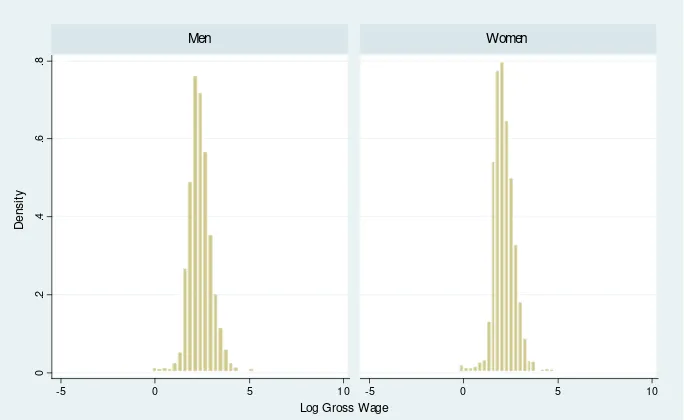
As we can see a spike at zero in both distributions showing the non par-ticipation but more pronouncing spike appears for women. The distribution of working hours implies that the men tend to work mostly around the mean value of 35 hours per week (apart from non participation) whereas the women’s working distribution unfold a form of part time employment. Probably there exists a degree of ‡exibility in employment contracts on female labor market that causes relatively non negligible distribution of working hours within the part-time region. The gross hourly wage of employed women in the sample was 10.91 GBP what is less than the gross hourly wage of employed men that amounts 15.40 GBP, on average. The distribution of the gross hourly wage of employed men shows greater inequality in comparison with women, where more than 70 percent of men are below the mean value of gross hourly wage. The skewness of gross hourly wage distribution for women is less emphasized with about 60 percent of women are below the mean value of gross hourly wage.

0

.2

.4

.6

.8

-5 0 5 10 -5 0 5 10

Men Women

D

e

n

s

ity

Log Gross Wage

Figure 1: Histogram of the gross hourly wage for men and women

5

Results

This section provides the results from the Heckman model for the wage equation and the results from the participation model. I analyze the results from both models where in addition for the probit model, the marginal e¤ects is computed and discussed.

5.1

Heckman sample selection model results

It is crucial to check whether the selection in Heckit model is based on unobserv-able characteristics. If the error terms, 1and 2, are correlated in the Heckit

model after conditioning on other right hand side variables, then the selection two step approach is justi…ed. The participation and wage equation implies that unobserved factors that make someone to work more may also make them to work longer that it would be predicted. The presence of unobservable char-acteristics has been tested in the model and the results con…rmed presence of sample selection bias.

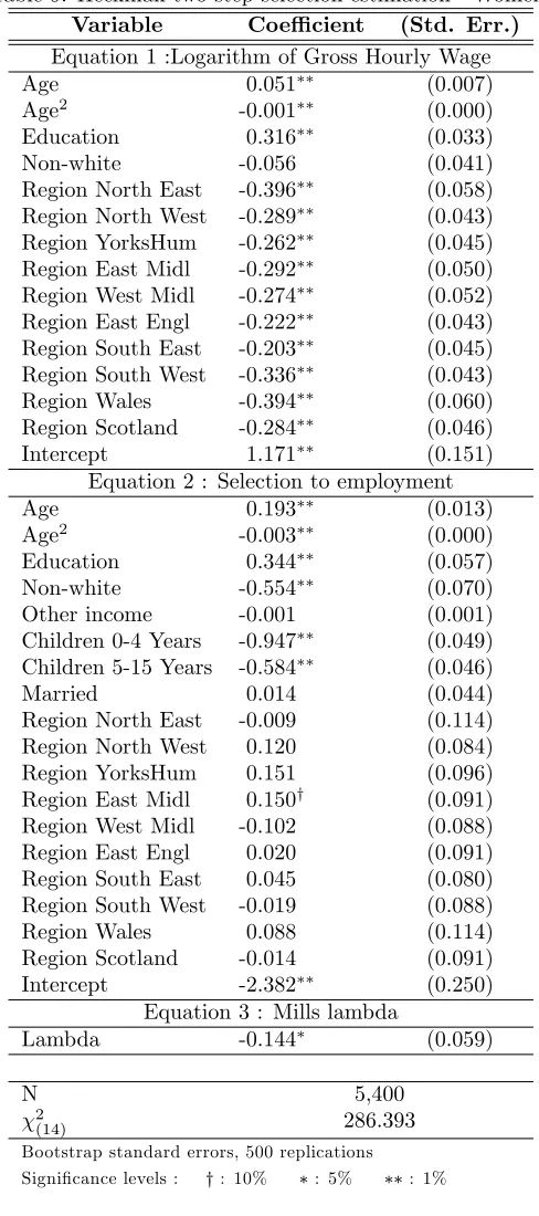
Table 8 and table 9 presents the estimated parameters in log-linear model for the gross wage, that take into account for potential sample selection bias24_. Us-ing the Heckit model I focus on modelUs-ing logarithmic wage for those in employ-ment. The inverse Mills ratio term is statistically signi…cant for men,z= 3:10

and for women,z= 2:61which implies the presence of sample selection bias. Moreover, the magnitude of the inverse Mills ratio term is almost one for men,

^ = 0:985and it is lower for women,^ = 0:232. The t-statistics on regional indicators in the selection equation are mostly insigni…cant either for men or women, which implies that regions does not a¤ect the participation in labor force. However, the regional binary variables are highly signi…cant in wage equation for both genders. All demographic variables except the educational binary variable for women and other income variable are statistically signi…cant and therefore have their impact on the wage o¤ered. The presence of children in the household does not seem to have an e¤ect for male participation25_in the market. In contrast with men, the presence of children has a negative and signi…cant e¤ect for women. Regarding marital status, there is no e¤ect on participation for either men or women.

After predicting the logarithmic wages for men and women by the Heckit model, one can make the comparison of predicted wages and actual wages for those that participate in the labor market. The results for working men in the table 10 imply that the average predictions of the logarithmic wages from the Heckit model are exactly the same in mean as the actual wages. The last line

2 4_{The OLS standard errors and heteroscedasticity robust standard errors in the Heckit}

model are not correct because the error term, i, su¤ers from heteroscedasticity since the

truncated variance of the dependent variable is heteroscedastic. Although, Heckman (1979) provided the expressions for the correct standard error they are not used in estimation. Rather, I used the empirical bootstrap method with 500 replications to correct for the heteroscedas-ticity of errors.

2 5_{The presence of children until 4 years old has a statistically signi…cant e¤ect at 10 percent}

in table 10 shows that without taking the sample selection bias into account, on average logarithmic wages for working men are over predicted. The same predictions have been made for woman and the results are summarized in table 11. Again, the average predictions of the logarithmic wages for women from the Heckit model are perfectly matching with the mean of observed wages. Comparing the mean linear predictions of the logarithmic wage for women with the actual logarithmic wage reveals that the former wages are over predicted on average. When comparing the mean of linear over prediction from the mean of actual wages by gender, for women this accounts 0.45 GBP while for men accounts 1.72 GBP.

The Heckit conditional wage predictions are made for all individuals in the sample but they can be compared only with observed wages for those in em-ployment. However, we can be interested in comparing the mean of wages for all men and women whether they participate in paid work or not. The mean of the Heckit conditional predictions of wages and the mean of observed wages for all men in the sample are presented in table 1226_{. One can note that the} predictions from the Heckit model for the gross hourly wages are similar to the mean of observed gross hourly wages. The mean of the Heckit predicted gross hourly wage for those men in paid work are larger for about 2.53 GBP than the same prediction for all men in the sample. This result is nevertheless ex-pected because when predicting the gross hourly wage for all men by the Heckit method, the cumulative distribution function that measures the probability of being in the labor force is smaller than one.

Comparing the mean gross hourly wages predicted by the Heckit and actual gross hourly wage shows that these two are very similar for women. On average the Heckit predicted gross hourly wage for employed women are larger then the Heckit prediction by about 2.63 GBP. These results are presented in the table 13.

5.2

The participation decision model results

The wage equation from the Heckit model predicted the wages for non-workers whose wages were not observed. The actual and predicted gross hourly wages were used to derive the e¤ective net hourly wages27_{that will be used as the main} regressor in estimating the labor force participation rates. The probability of working is estimated with the probit model and the results are presented in the table 14 and table 15 for the gross wage speci…cation and in the table 16 and table 17 for the net e¤ective wage speci…cation.

There are two speci…cations of the probit model, one with the logarithmic gross hourly wage and the other with the logarithmic e¤ective net hourly wage. Comparing the goodness of …t with 2 _{statistics (of the Wald test whether}

all coe¢cients except the constant) across two speci…cations of a model, the

2 6_{One should note that these predictions are in wage levels not in the logarithm. For}

comparison, observed wage for those who are determined by participation equation as non-participants, are set to zero.

speci…cation with the e¤ective net wage performs approximately the same as the speci…cation with the gross wage and that is for both gender. The comparison of …t based on the pseudo-R2 _{shows equivalence for both speci…cations within the}

gender but marginally better performance for women when comparing between gender. The positive sign on wage coe¢cients for men and negative coe¢cients for women indicate that the probability of supplying labor will increase for men and decrease for women if there is a change in the wage. One reason for that might be that men will substitute away leisure for work due to greater substitution than income e¤ect, and women will do the opposite by substituting work for leisure due to greater income e¤ect. The positive sign on age coe¢cient implies that labor supply is increasing with age but there is a point above which the age has negative e¤ect on the probability of working (marginal decreasing returns on age are present). The e¤ect of education on probability of working is signi…cant only for women and positive impliying that educated women are more likely to work in contrast with women without education. The presence of children reduces men’s and women’s probability of employment and the e¤ect decreases with the children’s age. However, the presence of children older than four years has no e¤ect on men’s decision to work. As probably expected, non-labor income has negative e¤ect on the probability of employment, although the e¤ect is insigni…cant for women and marginally signi…cant for men. Positive coe¢cient on marital status indicates higher probability of working for married people than non-married, however there is no e¤ect for women. The probability of working increases for white men and women in contrast with non-whites’28_.

5.3

Elasticity results

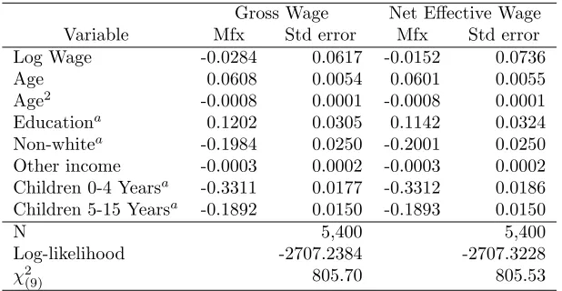
While one can draw inferences about the sign and signi…cance of the regressors from the probit model by looking at the coe¢cients, the magnitude of these e¤ects cannot be read directly. Therefore, the marginal e¤ects need to be calcu-lated at either at the mean or other interesting value of variables. The marginal probit e¤ects are not constant like in the usual OLS regression model but they di¤er in size due to the non-linearity of the probit model. After estimating the probit model for labor force participation, the marginal e¤ects are calculated and presented in the table 2 and table 3 for men and women, respectively.

These e¤ects were calculated at the means of the variables29_{. However,} the means of the marginal e¤ects computed for each individual is presented in addition. The …rst row of the table 2 and table 3 shows the wage semi-elasticity

2 8_{The e¤ects on country binary variables are not signi…cant for women. The joint and}

individual signi…cance of the binary variables, Wales and Scotland were checked by likelihood ratio test and z-statistics. The former test showed no signi…cant joint e¤ect at 10 percent signi…cance level for women’s sample.

2 9_{Marginal e¤ects of continuous regressors are computed by using the probability density}

of labor supply30_{. When comparing either the gross wage semi-elasticity or} the net e¤ective wage semi-elasticity across gender, they are both larger for men than for women. The gross wage has signi…cant e¤ect on male labor force participation decision implying that a one percent increase in gross hourly wage increases the probability of supplying labor by 0.0951 percentage point for men with the average characteristics in the sample.

In contrast with men, increasing the gross wage will reduce the probability of supplying labor for women by 0.0285 percentage point, however the e¤ect is not signi…cant. Calculating the mean marginal e¤ects31_{, by dividing the wage} semi-elasticities with the predicted probability of labor force participation at means of variables, the gross wage elasticities are 0.1046 and -0.0373 for men and women, respectively32_.

Evaluating the marginal e¤ect of additional age at the average value of vari-ables in the sample33 _{increases the probability of supplying labor for 0.02 and} 0.06 percentage point for men and women, respectively. The marginal dimin-ishing e¤ect of age is signi…cant and it present for men and women. While education does not have signi…cant e¤ect on male labor supply, its e¤ect is signi…cant and pronounced for women implying that the probability of being employed for women with at least high school educational attainment34 _{is by} 0.12 higher than for women without high school. The negative marginal e¤ect on race binary indicator implies that the probability of labor supply is higher by 0.09 and 0.20 for white men and women, conditional on the averages of other characteristics. The e¤ect of non-labor income, although not signi…cant for both genders, has the expected sign. The probability of supplying labor

3 0_{Wage semi-elasticity of labor supply,!, is de…ned as the following expression:}

!=@Pr(IN LF = 1)

@logwage =

@Pr(IN LF = 1)

@wage wage

that can be interpreted as the wage marginal e¤ect on the probability of supplying labor,

mf x=@Pr(IN LF = 1)

@logwage = ( ln(wage) +X )

where ( )denotes the standard normal density function. We can interpret these e¤ects as:

a one percent increase in wage, increases the probability of supplying labor by(1=100) mf x:

3 1_{Mean wage marginal e¤ect or wage elasticity can be expressed as:}

= @Pr(IN LF = 1)

@wage

wage

Pr(IN LF = 1)

= !

Pr(IN LF = 1)

The wage elasticity is calculated by using ! and the predicted probability of labor force

participation,Pr(IN LF = 1).

3 2_{The wage elasticity for men is close to wage semi-elasticity because the predicted labor}

force participation is 0.9088 or 90.88 percent. While for women, the wage semi-elasticity is larger then the wage elasticity due to the predicted labor force participation of 0.7643 or 76.43 percent.

3 3_{The average age for men and women in the sample is approximately the same, that is 40}

years old.

Table 2: Marginal E¤ects-Men

Gross Wage Net E¤ective Wage

Variable Mfx Std error Mfx Std error

Log Wage 0.0951 0.0516 0.1043 0.0525

Age 0.0236 0.0037 0.0232 0.0041

Age2 _{-0.0003 0.0000 -0.0003 0.0000}

Educationa _{0.0102 0.0175 0.0090 0.0172}

Non-whitea _{-0.0944 0.0225 -0.0973 0.0220}

Other income -0.0006 0.0002 -0.0006 0.0002

Children 0-4 Yearsa _{-0.0272 0.0154 -0.0271 0.0152}

Children 5-15 Yearsa _{-0.0138 0.0111 -0.0138 0.0117}

Marrieda _{0.0760 0.0114 0.0761 0.0114}

N 4,392 4,392

Log-likelihood -1383.6852 -1383.6771

2

(9) 275.92 275.93

Notes: Marginal e¤ects computed at the means of regressors. Discrete change denoted by a. Statistical signi…cance is calculated using bootstrap standard errors, 500 replications.

Table 3: Marginal E¤ects-Women

Gross Wage Net E¤ective Wage

Variable Mfx Std error Mfx Std error

Log Wage -0.0285 0.0617 -0.0152 0.0730

Age 0.0611 0.0054 0.0603 0.0054

Age2 _{-0.0008 0.0001 -0.0008 0.0001}

Educationa _{0.1205 0.0299 0.1146 0.0285}

Non-whitea _{-0.1988 0.0250 -0.2006 0.0238}

Other income -0.0003 0.0002 -0.0003 0.0003

Children 0-4 Yearsa _{-0.3318 0.0187 -0.3319 0.0184}

Children 5-15 Yearsa _{-0.1900 0.0154 -0.1898 0.0154}

Marrieda _{0.0034 0.0132 0.0035 0.0130}

N 5,400 5,400

Log-likelihood -2707.2384 -2707.3228

2

(9) 805.70 805.53

decreases for men and women that have children while the e¤ect is far more intense for women than the men. Probability that a female with the average characteristics in the sample supply labor is lower by 0.33 if the children below for years old is present in the household. While marital status has no signi…cant e¤ect for women‘s labor supply, married men‘s have higher probability of being participating in the labor force than unmarried.

The following results are based on the second speci…cation using net ef-fective wage rate and evaluating marginal e¤ects at the average of regressors. The semi-elasticities of labor force participation with respect to net e¤ective wage are larger than the semi-elasticities with respect to gross wage, for men and women. The e¤ect is signi…cant for men and implies that a one percent increase in net e¤ective wage increases the probability of supplying labor by 0.1043 percentage point. For women the semi-elasticity is negative, implying that one percent rise in net e¤ective wage decreases the probability of labor supply by 0.0152 percentage point. However, the e¤ect for women is insignif-icant at even 10 percent signi…cance level. The net e¤ective wage elasticities calculated as mean marginal e¤ects are 0.1148 and -0.0199 for men and women, respectively. Again, the wage elasticity is closer to wage semi-elasticity for men than for women because the predicted probability of labor force participation is larger for men than for women. The marginal e¤ects of socio-demographic characteristics on labor force participation are the same magnitude and sign in net e¤ective wage speci…cation as for the gross wage speci…cation. The marginal e¤ect of education in net e¤ective wage speci…cation is marginally lower than with gross wage speci…cation, for both gender. The probability of supplying labor for men and women with white ethnic background is marginally larger in net wage speci…cation than with gross wage speci…cation in comparison with non-whites.

Analyzing the wage elasticities for di¤erent wage speci…cation, the net ef-fective wage elasticities are larger than the gross wage elasticities for both gen-der, although wage elasticities show no signi…cant e¤ect on labor supply for women. One reason for greater net e¤ective wage elasticities can be determined by greater equality of net e¤ective wage distribution among the individuals. This e¤ect can be achieved by marginal e¤ective tax rate created by a state or local authorities when seeking for a greater contributions in social transfers and progressive taxation of personal income.

Hypothetically assuming that all individuals in male sample and female sam-ple are married, the following results are obtained by computing the wage semi-elasticity of labor supply. That is to say, these marginal e¤ects are measuring the labor supply response to both wage speci…cations when there is no unmar-ried male or female in the sample. Comparison of the predicted probabilities of labor supply for married individuals are than compared to the predicted proba-bilities of labor supply that are measured on the averages of the variables. The di¤erence between the marginal response of two wage speci…cations in hypo-thetical example stays with the same sign and magnitude35 _{as in the di¤erence}

Table 4: Marginal E¤ects for Married-Men

Gross Wage Net E¤ective Wage

Variable Mfx Std error Mfx Std error

Log Wage 0.0718 0.0361 0.0787 0.0394

Age 0.0178 0.0033 0.0175 0.0033

Age2 _{-0.0003 0.0000 -0.0002 0.0000}

Educationa _{0.0078 0.0138 0.0068 0.0140}

Non-whitea _{-0.0743 0.0195 -0.0766 0.0187}

Other income -0.0004 0.0002 -0.0004 0.0002

Children 0-4 Yearsa _{-0.0207 0.0111 -0.0207 0.0117}

Children 5-15 Yearsa _{-0.0104 0.0081 -0.0105 0.0083}

N 4,392 4,392

Log-likelihood -1383.6852 -1383.6771

2

(9) 275.92 275.93

Notes: Marginal e¤ects computed at the means of regressors. Discrete change denoted by a. Statistical signi…cance is calculated using bootstrap standard errors, 500 replications.

Table 5: Marginal E¤ects for Married-Women

Gross Wage Net E¤ective Wage

Variable Mfx Std error Mfx Std error

Log Wage -0.0284 0.0617 -0.0152 0.0736

Age 0.0608 0.0054 0.0601 0.0055

Age2 _{-0.0008 0.0001 -0.0008 0.0001}

Educationa _{0.1202 0.0305 0.1142 0.0324}

Non-whitea _{-0.1984 0.0250 -0.2001 0.0250}

Other income -0.0003 0.0002 -0.0003 0.0002

Children 0-4 Yearsa _{-0.3311 0.0177 -0.3312 0.0186}

Children 5-15 Yearsa _{-0.1892 0.0150 -0.1893 0.0150}

N 5,400 5,400

Log-likelihood -2707.2384 -2707.3228

2

(9) 805.70 805.53

in the marginal responses measured at the average of variables. However, the magnitude of marginal e¤ects for both wage speci…cations are smaller when as-suming only married men relatively in comparison with the average value for marital status variable in the sample. The results are presented in table 4 and table 5.

A one percentage point rise in gross wage increases the probability of sup-plying labor by 0.0718 percentage point for men in the hypothetical example, while the same e¤ect was 0.0951 when measuring the e¤ect on the average of marital status variable. The disincentive e¤ect by comparing these two scenar-ios is 25 percent. For net e¤ective wage speci…cation, a one percent increase in wage for men, raises the probability of labor supply by 0.0787 in hypothetical case, while on the average of marital status variable the same e¤ect was 0.1043. The disincentive e¤ect of these two scenarios is 25 percent. The marginal wage e¤ects on the predicted probability of labor supply in the hypothetical scenario for women stay the same as the marginal wage e¤ects on the predicted proba-bility of labor supply when the e¤ects are calculated at the means of variables. The estimated e¤ects of other socio-demographic characteristics of labor force participation for both wage speci…cations and across genders, are the same sign and approximately the same size in two scenarios that were recently presented. Illustration of marginal e¤ects of marital status on labor supply over the whole sample distribution is presented by computing the predicted probabilities of labor force participation. Cumulative distribution function is evaluated at the sample means of regressors and with the two values for variable represent-ing marital status, where estimated coe¢cients of variables follow the coe¢-cients estimated from the probit model. Figures 3 and 4 presents the predicted probabilities as a function of wage for both wage speci…cations and across both genders. The marginal e¤ect of variable indicating the marital status is given by di¤erence between the two functions.The probability that the labor force participation will increase for men after marriage is substantially greater for men with low level of wages than those with high level of wages. However, over the whole wage distribution, the probability of supplying labor will be greater for married than for unmarried men. At around of net e¤ective wage level that equals 4 GBP (per hour), the estimated probability of supplying labor will be 72 percent for unmarried men and 85 percent for married men. At the wage level of around 15 GBP, the estimated probability of labor supply is 91 and 96 percent for unmarried and married men, respectively. The marginal change in the estimated probability of being employed does not di¤er for female marital status over the wage distribution. For every wage level the probability of being employed is higher for married than the unmarried women. At the net e¤ective wage level of 4 GBP the predicted probability of working is around 77 percent and it is marginally di¤erent between married and unmarried women. Interest-ingly, at the higher wage level of around 9 GBP, the predicted probability of working falls by approximately 1.5 percentage points for unmarried women and by 1.2 percentage points for married women.

.7 .75 .8 .85 .9 .95 P red ic ted labo r for c e pa rt ic ipat ion

5 10 15 20

Gros s W age

C df (Mar ried )

C df (U nmarr ied)

.7 .75 .8 .85 .9 .95 P red ic ted labo r for c e pa rt ic ipat ion

4 6 8 10 12 14

N et effec tiv e W age

C df (Mar ried )

C df (U nmarr ied)

Figure 2: Predicted labor force participation rates for married and unmarried men .75 .76 .77 .78 .79 P redi c ted labor for c e par tic ipa tion

4 6 8 10 12 14

G ros s W age

C df (Married)

C df (U nmar ried)

.7 55 .76 .7 65 .77 .7 75 P redi c ted labor for c e par tic ipa tion

4 6 8 10

N et effec tiv e W age

C df (Married)

C df (U nmar ried)

Table 6: Marginal E¤ects by Gross Wage and Gender

Wage Men Women

Quartile Wage (GBP) Mfx Wage (GBP) Mfx

Q1 Below 8.2293 0.7255 Below 6.2644 0.0660 Q2 Below 9.4743 0.8526 Below 7.1832 -0.4504 Q3 Below 10.3399 0.5585 Below 7.7168 -0.3444 Q4 Above 10.3399 0.0904 Above 7.7168 0.0283

All 0.1047 -0.0373

Notes: Averages of marginal e¤ects in each quintile. Statistical signi…cance is calculated using bootstrap standard errors, 10 replications.

The marginal e¤ects presented so far are evaluated at the means of the variables to illustrate the partial e¤ects of an individual with the average char-acteristics on the probability of labor supply. Table 6 and table 7 represents the estimated wage semi-elasticities for given quartiles of hourly wage.

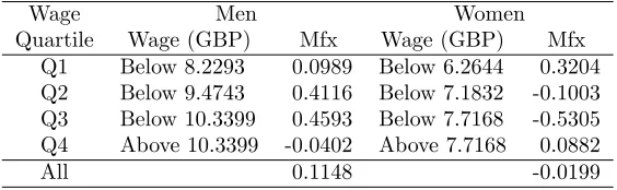
The semi-elasticities in these two tables are computed within quartiles on averages of regressors and at the end total averages of the marginal e¤ects are evaluated for each individual. When comparing the total marginal e¤ects presented in the last row of these two tables with the marginal e¤ects in the table 2 and table 3, we can notice that the di¤erence in computing marginal e¤ects at means or means of marginal e¤ects is negligible. Computing the marginal e¤ects at means is preferable for having the correct standard errors that were obtained through the bootstrap method. The wage semi-elasticity decreases with the wage levels for both speci…cations and both genders when comparing the …rst and the fourth quartile but the results for the second and third quartile are more ambiguous. For both speci…cations and both genders, the wage elasticities in the second and third quartiles are more pronounced than the other quartiles. The cross-quartile di¤erences are more pronounced in absolute values for men than for women for gross wage speci…cation but the opposite is true for the net e¤ective wage speci…cation. The semi-elasticity of labor force of men with respect to the e¤ective net wage in the …rst quartile is, in absolute terms more than twice the wage semi-elasticity in forth quartile, while for gross wage speci…cation the marginal e¤ect in …rst quartile is eight times the response in fourth quartile. A one percent increase in the gross wage raises the labor force participation of men in the …rst quartile by 72.55 percentage points, which is almost seven times the overall average marginal response. In the net e¤ective wage speci…cation, a one percent increase in the wage, increases the labor force participation of men in the …rst quartile by 9.89 percentage points, which is below the overall average marginal response.

Table 7: Marginal E¤ects by Net E¤ective Wage and Gender

Wage Men Women

Quartile Wage (GBP) Mfx Wage (GBP) Mfx

Q1 Below 8.2293 0.0989 Below 6.2644 0.3204 Q2 Below 9.4743 0.4116 Below 7.1832 -0.1003 Q3 Below 10.3399 0.4593 Below 7.7168 -0.5305 Q4 Above 10.3399 -0.0402 Above 7.7168 0.0882

All 0.1148 -0.0199

Notes: Averages of marginal e¤ects in each quintile. Statistical signi…cance calculated using bootstrap standard errors, 500 replications

in fourth quartile, while for gross wage speci…cation the marginal response in the …rst quartile is three times greater that the response in fourth quartile. A one percent increase in the gross wage raises the labor force participation of men in the …rst quartile by 6.60 percentage point, which is twice in absolute terms than the overall average marginal e¤ect. Considering the net e¤ective wage speci…cation, a one percent increase in the wage increases the labor force participation of women in the …rst quartile by 32.04 percentage point, which is, in absolute terms is about sixteen times the overall average marginal ef-fect.The wage -elasticity of women is distributed more equally within quartiles with the gross wage semi-elasticity ranges in the absolute terms from 0.0660 in the …rst quartile to 0.0283 in the forth quartile, the net e¤ective semi-wage elas-ticity range is from 0.3204 to 0.0882 in absolute terms. The di¤erence between the gross and net e¤ective wage elasticities measured with the overall average marginal e¤ect is an evidence for the Britain‘s improving welfare system. The system of taxes, social security contributions and social bene…ts encourages the labour force participation more than in the case when this incentives will not be present. Computing the di¤erence between the marginal e¤ects for the gross and net e¤ective wage speci…cations, the tax-bene…t system encouragements are larger for women36 _{than for men. The marginal e¤ect of the e¤ective net wage} on labor force participation is larger than the e¤ect of the gross wage by 47 per-cent for women while both elasticities are negative. This means that the welfare system disincentives are lower than if we consider no existence of such a system. For men, the marginal e¤ect of net e¤ective wage is larger than the e¤ect of the gross wage by 10 percent. In contrast with women, this net marginal e¤ect is positive for males, implying the existence of welfare incentives. The interpre-tation of the di¤erences between the two wage speci…cations across the wage quartiles is more ambiguous because for men all four wage quartiles show the disincentive e¤ect of welfare system while the overall e¤ect shows the opposite. However, the comparison of the results from overall marginal e¤ect di¤erences

3 6_{However, this is only true when measuring the di¤erence in a way of reducing the}