Estimates of the Steady State Growth Rates for Ireland

Munich Personal RePEc Archive

Estimates of the Steady State Growth

Rates for Ireland

Casadio, Paolo and Paradiso, Antonio and Rao, B. Bhaskara

22 April 2011

Estimates of the Steady State Growth Rates for Ireland

Paolo Casadio [email protected]

Intesa Sanpaolo Bank Group, Risk Management, Rome (Italy)

Antonio Paradiso [email protected]

Department of Economics, University of Rome La Sapienza, Rome (Italy)

B. Bhaskara Rao [email protected]

School of Economics and Finance, University of Western Sydney, Sydney (Australia)

Abstract

This paper estimates the steady state growth rate for Ireland with an extended version of the Solow

(1956) growth model. We show that the education and trade openness have played an important role

to improve the long-run growth rate. Policies to further improve the long-run growth rate are

suggested.

Keywords: SSGR, Economic Growth, Trade Openness, Education, Ireland.

1. Introduction

The Irish economy during the second part of 1990s was one of the most successful in the OECD. In

the period 1995-2005 GDP grew at an average rate of 7.7%, well far ahead of many other industrial

economies. Ireland relies heavily on trade and foreign investment, with the combined value of

import and exports equivalent to above 140% of GDP. Using the index of trade openness (import +

exports as percentage of GDP) Ireland in 2010 was one of the most open economies in the OECD

area after Belgium, Hungary, Luxembourg, and Slovak Republic. The time-series data reveals a

growing trend toward openness after the 1970s and since its membership in the European Economic

Community. Another characteristic of Ireland is the steep rise in the educational attainment since

the 1990s, which brought Ireland in line with countries with high historical level of education.

According to the Barro and Lee (2010) dataset, Ireland is a leading country in education, in line

with schooling levels in Sweden, Germany and the Republic of Korea.

These considerations suggest that these variables have played an important role in explaining the

long-term growth rate of Ireland and its higher performance. We investigate this aspect with an

extended version of Solow (1956) growth model incorporating education and trade openness as key

variables of its long-run growth. Our approach broadly follows the specification and methodology

in Rao (2010) and Paradiso and Rao (2011).

2. Specification of the model

The starting point is the well-known Cobb-Douglas production function:

1

t t t

Y

A K L

(1)

where Y is for output, K for stock of capital and A is the stock of knowledge. Following Rao (2010)

and Paradiso and Rao (2011) we assume the following general evolution for A, as a simple function

of two variables S and Z for schooling and/or openness.

2 1 2

0

iZ Tit St St

t

A

A e

(2)

Transforming (1) into its intensive form, substituting (2) for A_t, and taking its logs gives:

2

0 1 2

where

y

( / )

Y L

and

k

(

K L

/ )

. In the steady state, when

ln

k

0

, the Steady State

Growth Rate (SSGR) is equal to the growth rate of the stock of knowledge (

ln

A

). There are two

ways to measure the SSGR. One restrictive method considers all the changes in the variables as

zero, whereas in a less restrictive version only

ln

k

0

. The first one may be treated as the very

long run growth rate and the second as the growth rate in the intermediate period. We call the first

as SSGR1 and the second as SSGR2 and are as follows.

1

_{i it}

SSGR

Z

(4)

1 2

2

_{i it}

+

_{i it}

+

_t

+2

_{t t}

SSGR

Z

T

Z

S

S

S

₍₅₎

We make use of both of these measures of SSGR and try to understand the potential factors

influencing the SSGRs and how policy can improve them.

3. Empirical Estimates

Yearly data from 1960 to 2010 are used to estimate the long-run relationship in equation (3). Our

selected growth-enhancing variables are: trade openness (TRADE) and human capital index (HKI).1

Definitions of variables and sources of data are in the appendix. Three estimations techniques are

used, which are the Fully Modified OLS (FMOLS), Canonical Cointegrating Regression (CCR) and

Dynamic OLS (DOLS). These estimators deal with the problem of second-order asymptotic bias

arising from serial correlation and endogeneity and they are asymptotically equivalent and efficient.

Two dummies are added in the estimations and are discussed in appendix.

Our estimation strategy is the following. We estimate the long-run relationship with these three

methods and if all the results are similar and plausible, we verify the existence of the cointegrating

relationship with the Engle-Granger (EG) residual test. If the tests confirm the existence of the

long-run relationship, we construct an Error Correction Model (ECM). Then we study the factor loading

and test for correct specifications i.e., we test for the normality, absence of autocorrelation, and

absence of heteroskedasticity in the residuals.

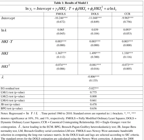
In the first model, shown in Table 1, equation (3) is estimated with

Z

_1t

HKI

_t = St. The results are

good except for the coefficient of capital

,

which is not statistically significant in the estimates

1

We have also included investment ratio (IRAT) as an additional determinant of SSGR but its coefficient was

with FMOLS and DOLS, and very low compared to its stylized value of one third in the growth

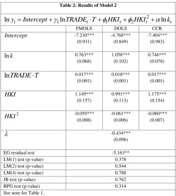
accounting exercises. Therefore, we estimated model 2 in which HKI is replaced with lnTRADE as

the determinant of SSGR. That is,

Z

_1t

ln

TRADE

_t

, and

S

_t

HKI

_t. The results are in Table 2

and it can be seen that all estimates are significant but the coefficient for capital ( ) is above

[image:5.595.54.548.217.696.2]

unity in DOLS estimation and this is implausible.

Table 1: Results of Model 1

2

1 1 2

ln

y

_t

Intercept

HKI T

_t

HKI

_t

HKI

_t

ln

k

_t

FMOLS DOLS CCR

Intercept -10.246*** (0.672) -11.048*** (0.849) -9.965*** (0.756)

lnk 0.065

(0.045)

0.039 (0.104)

0.093* (0.053)

HKI T 0.003***

(0.000) 0.003*** (0.000) 0.003*** (0.000) HKI 1.365*** (0.112) 1.499*** (0.300) 1.330*** (0.116) 2 HKI -0.074*** (0.006) -0.081*** (0.016) -0.073*** (0.005) -0.806*** (0.135)

EG residual test -5.027**

LM(1) test (p-value) 0.775

LM(2) test (p-value) 0.800

LM(4) test (p-value) 0.661

JB test (p-value) 0.478

BPG test (p-value) 0.636

[image:6.595.117.478.127.529.2]

Table 2: Results of Model 2

2

1 1 2

ln

y

_t

Intercept

ln

TRADE T

_t

HKI

_t

HKI

_t

ln

k

_t

FMOLS DOLS CCR

Intercept -7.210*** (0.931) -4.768*** (0.849) -7.404*** (0.983)

lnk 0.763***

(0.068)

1.058*** (0.102)

0.746*** (0.078)

ln

TRADE T

0.017*** (0.001) 0.018*** (0.001) 0.017*** (0.001) HKI 1.149*** (0.157) 0.991*** (0.113) 1.175*** (0.154) 2 HKI -0.059*** (0.008) -0.061*** (0.006) -0.060*** (0.007) -0.434*** (0.096)

EG residual test -5.163** LM(1) test (p-value) 0.378 LM(2) test (p-value) 0.544 LM(4) test (p-value) 0.788 JB test (p-value) 0.762 BPG test (p-value) 0.314 See note for Table 1.

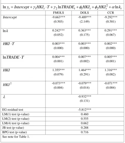
In model 3 we also include both HKI and lnTRADE as determinants of SSGR. In this case

1 2

,

,

ln

t t t t t t

S

HKI Z

HKI Z

TRADE

such that equation (3) becomes:

2

0 1 2 1 2

ln

y

_t

ln

A

HKI T

_t

ln

TRADE

_t

HKI

_t

HKI

_t

ln

k

_t

(6)

Note that there is an additional term for education ( HKI T) compared to the specification in

model 2. This implies that some of the non-linear effects of HKI are offset by the underlying trend

in HKI, which may be due to improvements in the quality of education over time. The results are in

Table 3 and are impressive. All the coefficients are statistically significant, the coefficient of capital

is close to one third, the residual tests (EG) confirm the existence of a long-run relationship and

of SSGR in equations (4) and (5). The plots of the two measures of SSGR for model 3 and the

actual growth of output per worker (DLYL) are in Figure 1. SSGR1 is the very long run growth rate

when changes in all variables are zero. It is smooth and shows a mild upward trend. SSGR2 is the

steady state growth rate in the intermediate period, when net investment is zero i.e., lnk 0, but

changes in HKI and TRADE are not zero. SSGR2 is close to DLYL. More importantly, SSGR2

shows the 2000s weakness of the economy although the actual growth rate is still over 2% in

[image:7.595.89.508.241.719.2]

2000-2002 period.

Table 3: Results of Model 3

2

1 2 1 2

ln

y

_t

Intercept

HKI T

_t

ln

TRADE

_t

HKI

_t

HKI

_t

ln

k

_t

FMOLS DOLS CCR

Intercept -9.663*** (0.503) -9.489*** (2.149) -9.292*** (0.581)

lnk 0.242***

(0.052)

0.363*** (0.175)

0.291*** (0.067)

HKI T 0.003***

(0.000)

0.003*** (0.000)

0.002*** (0.000)

ln

TRADE T

0.004*** (0.001) 0.007*** (0.002) 0.005*** (0.001) HKI 1.355*** (0.079) 1.464*** (0.291) 1.316*** (0.082) 2 HKI -0.073*** (0.004) -0.079*** (0.014) -0.071*** (0.004) -0.932*** (0.131)

EG residual test -5.812***

LM(1) test (p-value) 0.460

LM(2) test (p-value) 0.555

LM(4) test (p-value) 0.662

JB test (p-value) 0.288

BPG test (p-value) 0.716

[image:8.595.157.438.118.293.2]

Figure 1: SSGR from Model 3

-3.0% -2.0% -1.0% 0.0% 1.0% 2.0% 3.0% 4.0% 5.0% 6.0% 7.0%

DLYL SSGR1 SSGR2

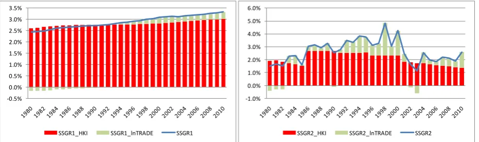
The contribution of HKI and TRADE to SSGR1 and SSGR2 are in Figure 2. In both cases the steady

state growth rate is mainly explained by HKI. It is interesting to note that the contribution of

TRADE is slightly negative in the early 1980s but later became positive with the exception for 2003

for SSGR2. This may be due to the high protectionist tariffs, which were phased out and replaced

after the mid 1980s with the more moderate tariffs of the European Union (EU). Ireland benefited

both from free trade within the EU and from lower EU tariffs. In SSGR2 the contribution of HKI to

the long run growth rate has been decreasing since 1990, offset by an increasing contribution of

TRADE. Only after 2000both contributions become smaller, reducing the rate of growth of the

economy in the following years.

Figure 2: Contributions of SSGR1 and SSGR2 to Growth

-0.5% 0.0% 0.5% 1.0% 1.5% 2.0% 2.5% 3.0% 3.5%

SSGR1_HKI SSGR1_lnTRADE SSGR1

-1.0% 0.0% 1.0% 2.0% 3.0% 4.0% 5.0% 6.0%

[image:8.595.58.524.566.704.2]

Although SSGR is still very high in Ireland, our estimates suggest that further improvements can be

made by improving education through job training schemes or by increasing the openness of the

markets. An increase of 1% in both HKI and TRADE will produce an increase of 0.6% in SSGR1.

SSGR2 is less sensitive to HKI and TRADE. An increase of TRADE by 5% will increase SSGR2

by only 0.1%.

4. Conclusions

This paper used an extended Solow (1956) growth model to estimate the long run and medium term

growth rates for Ireland. It is found that these two growth rates depend on the openness of the

economy and education and the latter seems to be the dominant determinant of the two growth

rates. The long run growth rate has shown a mild upward trend increasing from about 2.25% in the

early 1980 to 3% by 2010. The medium term growth rate showed some fluctuations and is below

the long term growth rate since the early 2000s. If the Irish economy is made more open and the

education levels are increased, both the long run and medium term growth rates will be closer and

Data Appendix

Y = Real GDP; L = Employment (Total economy); HKI = Human Capital Index measured as

average years of education; IRAT = Ratio of investment to GDP; TRADE = Ratio of imports plus

exports to GDP.

All data, excluding HKI, are taken and constructed from AMECO-EUROSTAT database. HKI is

taken from Barro-Lee (2010) database.

Dummy variables

Dummy for the second half of 1960s and dummy for the 2008-2009 financial crisis. The dummy for

1960s corresponds to a dummy for the years 1965-1966. These years corresponds to a brake in the

high growth rates of 1960s (in the period 1965-1966 the average growth rate was 1.4% against an

References

Barro, R., and Lee, J. (2010) A new data set of education attainment in the world, 1950-2010,

NBER Working Paper No. 15902. Available at http://www.barrolee.com/data/dataexp.htm (Accessed 29 April 2011).

Paradiso, A., and Rao, B. B. (2011) How to offset the negative trend growth rate in the Italian

economy?, Applied Economics Letters, iFirst, DOI: 10.1080/13504851.2010.54306.

Rao, B. B. (2010) Time-series econometrics of growth-models: A guide for applied economists,

Applied Economics, 42, 73-86.

Solow, R. M. (1956) A contribution to the theory of economic growth, Quarterly Journal of