The Development of Regression Models to Estimate Routine Maintenance Costs for State Highway Infrastructure

(1)

http://www.scirp.org/journal/jtts ISSN Online: 2160-0481

ISSN Print: 2160-0473

The Development of Regression Models to

Estimate Routine Maintenance Costs for

State Highway Infrastructure

Hualiang (Harry) Teng

1

, Monika Hagood

1

, Yathi V. Yatheepan

2

, Yuyong Fu

3

, Haiqing Li

4

1_{Department of Civil and Environmental Engineering, University of Nevada, Las Vegas, USA} 2_{Nevada Department of Transportation, Carson City, USA}

3_{Tianjin Huaxia Architectural Design Co., Ltd., Tianjin, China} 4_{Transportation Institute of Inner Mongolia University, Hohhot, China}

Abstract

Literature review indicates that most studies on pavement management have been on reconstruction and rehabilitation, but not on maintenance; this includes routine, corrective and preventive maintenance. This study developed linear regression mod-els to estimate the total maintenance cost and component costs for labor, materials, equipment, and stockpile. The data used in the model development were extracted from the pavement and maintenance management systems of the Nevada Depart-ment of Transportation (NDOT). The life cycle maintenance strategies adopted by NDOT for five maintenance prioritization categories were used as the basis for de-veloping the regression models of this study. These regression models are specified for each stage of life-cycle maintenance strategies. The models indicate that age, traf-fic flow, elevation, type of maintenance, maintenance schedule, life cycle stage, and the districts where maintenances are performed all are important factors that influ-ence the magnitude of the costs. Because these models have embedded the road con-ditions into the life-cycle stage and type of maintenance performed, they can be easi-ly integrated into existing pavement management systems for implementation.

Keywords

Highway Infrastructure Routine Maintenance, Regression Modeling

1. Introduction

Over the past decade or so, the population in Nevada has increased dramatically,

espe-How to cite this paper: Teng, H.L., Ha-good, M., Yatheepan, Y.V., Fu, Y.Y. and Li, H.Q. (2016) The Development of Regres-sion Models to Estimate Routine Mainten-ance Costs for State Highway Infrastructure. Journal of Transportation Technologies, 6, 339-359.

http://dx.doi.org/10.4236/jtts.2016.65030

Received: April 16, 2016 Accepted: September 27, 2016 Published: September 30, 2016

(2)

cially within and near the urban areas. This increase has resulted in the need to expand Nevada’s transportation system, particularly roadways. This expansion includes the construction of some new roadways; however, the greatest need involves improving nearly all existing major roadways. These improvements typically include addition-al lanes, turning lanes, sound waddition-alls, shoulder widening, upgrading older cross-section standards, adding guardrail, and more landscaping. New and improved existing road-ways have to be maintained, which adds to the demand for maintenance manpower, equipment, and materials.

Estimating the demand on the maintenance resources is needed when the mainten-ance districts of the Nevada Department of Transportation (NDOT) submit their main-tenance requests to headquarters. In turn, headquarters integrates the submissions and sends a request to state legislators for approval. Currently, NDOT’s Maintenance Divi-sion is responsible for the following maintenance activities:

1) Flexible Pavement, 2) Rigid Pavement, 3) Miscellaneous Concrete, 4) Roadside Infrastructure, 5) Roadside Cleanup, 6) Roadside Facilities, 7) Roadside Appurtenances, 8) Traffic Services,

9) Snow and Ice Control, 10) Bridge, and

11) Stockpile Production.

Ideally, the funding decision depends on the additional number of positions needed and the funding increase for equipment and materials for all these maintenance activi-ties over the life cycle of the highway system expansion. That decision could fully or partially meet the estimated demand for maintenance resources over the life cycles.

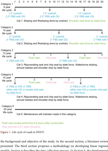
The objective of this research is to develop maintenance cost estimation models. These models estimate the total expected short-term and long-term maintenance bur-den required for NDOT. Short-term and long-term maintenance schedules for NDOT are shown in Figure 1. As can be seen in the figure, there is no preventive maintenance for maintenance prioritization Categories 1 and 2; on the other hand, there are more than one preventive maintenance activities between two constructions/rehabilitations for other prioritization categories.

In this study, linear regression models were developed for each individual stage of the life cycles in all these categories. These models estimated not only the annual main-tenance costs, but also estimated the component costs for manpower, materials, equip-ment, and stockpile. With this objective in mind, this study included a literature review on estimating maintenance cost. Data also were collected on maintenance cost and road characteristics. These data were used to develop linear regression models.

(3)

[image:3.595.191.542.73.564.2]

Figure 1. Life cycle of roads in NDOT.

the background and objective of the study. In the second section, a literature review is presented. The third section proposes a methodology on developing linear regression models. Section 4 describes the data collection process. In Section 5, the development of linear regression models for estimating annual maintenance costs is presented; this is followed by the last section, which summarizes the model development and identifies needs for future study.

2. Literature Review

(4)

from an additional unit of traffic loading. The study in [1] classified maintenance, re-habilitation and reconstruction (MR&R) costs models into five approaches:

1) The pavement management system (PMS) direct approach, 2) The simple roughness approach,

3) The econometric approach, 4) The cost allocation approach, and 5) The perpetual overlay indirect approach.

Among these five approaches, the most relevant ones to this study are the PMS ap-proach and the econometric apap-proach. A PMS usually consists of a database that records the history of MR&R work on a roadway system and a pavement performance model that can estimate the roadway surface condition, given the MR&R history and future maintenance policies and traffic usage of that roadway segment. Optimal procedures usually are applied to search for the optimal MR&R schedule. As a product of the op-timal procedure, maintenance costs can also be derived.

The econometric approach classified in [1] is to estimate a function that relates the total maintenance cost to influencing factors, such as traffic load, road geometry, pavement structure, and climate. It should be noted that there are only a few studies on estimating MR&R costs. However, the costs in these studies combined maintenance costs with rehabilitation and reconstruction costs. The most relevant study [2] used a regression modeling approach to study the impact of heavy trucks on maintenance cost. In their study, more than 1100 mile sections of highway were sampled randomly. Data including annual average daily traffic (AADT), maintenance cost, highway geometric information, and weather were collected from various sources and integrated into a single database, which was used to develop the regression model. The annual mainten-ance costs are related to AADTs of heavy trucks and passenger cars, age of pavement, pavement shoulder, temperature, maintenance location, the existence of a bridge, func-tional classification, and the district where a pavement section was located. It was found the maintenance cost incurred by heavy trucks was much higher than passenger cars; this has a significant implication to transportation policies, such as taxation.

In the 1990s, NDOT studied on various methods to estimate maintenance costs [3]. In that study, four techniques used in estimating maintenance costs were discussed ([3] [4]), which are:

1) Correlating annual maintenance costs to the present serviceability index (PSI) lev-el,

2) Correlating annual maintenance costs to the probability of their occurrence, 3) Establishing an overall annual maintenance cost for each treatment, and

4) Establishing a fixed-period, cumulative, annual maintenance cost for each treat-ment.

(5)

involved in pavement performance—for example, not every maintenance activity occur every year—the maintenance costs fluctuate significantly between years. Therefore, the second method correlates the annual maintenance costs to the probability of the occur-rence of maintenance activities. The third technique calculates the annual maintenance costs by considering the life of pavement after a certain treatment. The annual main-tenance costs are the average of the total mainmain-tenance costs over the year before next maintenance treatment. By the fourth technique, the annual maintenance costs consid-er the time since the last pavement treatment.

In NDOT’s study ([3][4]), the last technique was adopted. Note that all four tech-niques are not regression models that can consider the different characteristics of pave-ment, such as traffic load and road functional classification, which are critical in deter-mining the pavement conditions and the maintenance costs.

3. Methodology

In this study, regression models were developed for different maintenance costs, main-tenance prioritization categories for various highway routes, and different life-cycle stag-es. The maintenance costs were broken down into manpower, materials, equipment, and stockpile costs.

In NDOT, the highway routes are classified into five maintenance prioritization cat-egories, each with different maintenance strategies over their life cycles (see Figure 1) and road characteristics in terms of access control, traffic flow, etc. For the Category 1 routes, only one life-cycle stage is considered; it starts from reconstruction with “1.5'' coldmill, 2.5'' PBS with OG” and ends with another such reconstruction. Similar to the Category 1 route, only one life cycle stage is considered for Category 2 routes; it starts from and ends with “2'' coldmill, 2.5'' PBS with OG”. There are three life cycle stages for Category 3: After reconstruction, After Flush Seal, and After Chip Seal. Category 4 has four life cycles, which are: After Reconstruction, After Flush Seal, After First Chip Seal, and After the Second Chip Seal. In other words, there is one more Chip Seal treatment for Category 4 routes than for Category 3 routes.

There is no clear maintenance treatment pattern that has been adopted for Category 5. In this study, three life cycle stages are proposed for Category 5 routes: Beginning Stage (1st_{Stage), Middle Stage (2}nd_{Stage), and Last Stage (3}rd_{Stage), where the middle}

stage can be employed repeatedly.

Linear regression models were developed for each life cycle stage of these five differ-ent maintenance prioritization categories. The models can be written as:

1 2 2 3 3 , .

i i i k ki i

Y =β β+ X +β X + + β X +ε ∀i

The dependent variables Yi are the maintenance costs for total maintenance cost and

for man power, materials, equipment, and stockpile, separately. The Xi indicates the

(6)

4. Data Collection

The goal of data collection was to extract maintenance cost data, road section characte-ristics, and traffic flow data. The first step was to develop an inventory of roads main-tained by NDOT that could be used as a population for sampling. In the second step, time-space diagrams were developed for the selected roads, in which the history of maintenance activities on each selected road could be presented. The third step utilized the time-space diagrams to identify the road sections that showed uniform mainten-ance treatments. The fourth step involved extracting maintenmainten-ance cost data for selected road sections. In the last step, data on road characteristics were collected for the identi-fied road sections.

[image:6.595.198.554.542.687.2]

NDOT uses a pavement management system database that contains a data item for each maintenance prioritization category. This data item is used to extract the road in-ventory data for every road of each county in Nevada. Note that one road could be di-vided into multiple sections, each with a different maintenance prioritization. Main-tenance time-space diagrams present the mainMain-tenance tasks historically performed on a road. As shown in Figure 2, the x axis represents the years when maintenance occurred and the rehabilitation or reconstruction performed; the y axis indicates the locations where the maintenance activities happened on a road. Different colors are used to dif-ferentiate various maintenance tasks, which can be identified from NDOT’s PMS and maintenance management database. The maintenance work performed by NDOT’s work force that directly influence road performance is classified as: 1) Base & Surface Repair, 2) Hand Patching, 3) Machine Patching, 4) Maintenance Overlay, Inlay (Sche-duled Betterment), 5) Roadway Capital Improvements (Sche(Sche-duled Betterment), 6) Sand, 7) Fog/Flush, 8) Chip, 9) Scrub/Slurry, 10) Crack Filling, and 10) Cold Milling. From the colors, the road sections that experienced the same set of maintenance tasks historically can be easily distinguished. The time-space diagrams for prioritization Categories 3, 4 and 5 are presented with minor differences to distinguish them from those for Categories 1 and 2, because preventive maintenance tasks on these routes are different. These time-space diagrams were developed based on running an MS Excel program written using a Macro.

(7)

The mile-by-mile traffic flow data available in the PMS database varies over a given road section. Thus, averaging has to be performed for the mile-by-mile traffic flow data. When the length of road section is great, the mile-by-mile midpoint elevations on the road section may vary; in that case, the average of these mile-by-mile midpoint evalua-tion data needs to be derived. Usually, however, road characteristics data for the most recent years have the complete mile-by-mile midpoint elevation data. Other road cha-racteristics data—such as number of lane, type of road surface, and urban/rural—do not vary over the length of a road section; therefore, they can be collected by various methods. Maintenance cost data were extracted from the NDOT MMS database. To fa-cilitate the data extraction, a Microsoft spreadsheet program was developed.

5. Maintenance Cost Model Development

5.1. Maintenance Prioritization Category 1

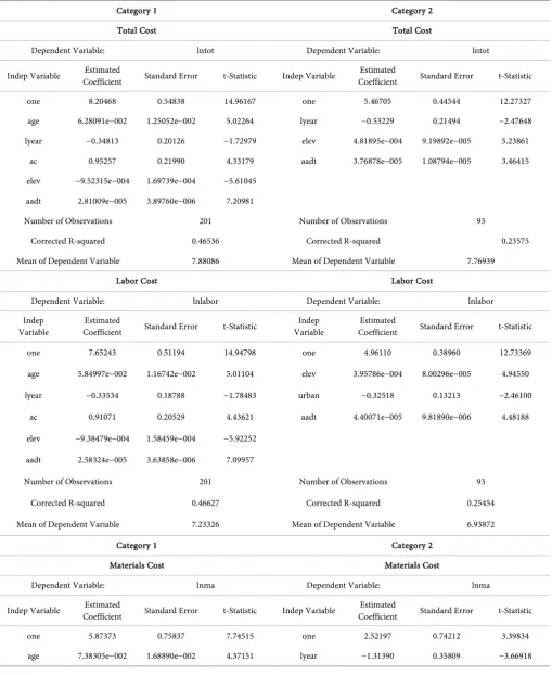
Linear regression models were developed for total maintenance cost and the compo-nent costs for labor, equipment, materials, and stockpiles. The results of these models are listed in Table 1. It can be seen from the table that the coefficient for the variable age is positive, which implies that the total maintenance cost increases with year. In the last year before a reconstruction, certain maintenance work may not be performed; thus, the coefficient for the last year indicator is negative. The coefficient for the factor “asphalt concrete” is positive, which indicates that the roads with an asphalt concrete surface incur more maintenance cost than rigid concrete pavement roads. The elevation of the road segment is also important to determine the amount of maintenance costs. The coefficient for the factor “elevation” is negative. This is because the data samples were from the Las Vegas area, where the roads of highways I-15 and US95 outside of the metropolitan area are at high elevations, and less maintained. The maintenance ac-tivities vary with the conditions of roads that are influenced by the amount of traffic rolling over them. The more vehicles travel on roads, the more deterioration results, which triggers more maintenance activities. The coefficient for “AADT” is positive, which is consistent with the study’s expectations. From Table 1, it can be seen that these influencing factors show similar impacts on labor, materials, and equipment costs.

When the total maintenance cost was analyzed, it was shown that the maintenance cost in the year when a reconstruction happened was significantly less than previous years. This observation can be validated from the model for labor costs, which implies that those maintenance activities involving expensive equipment and materials were not performed in a year during which major construction was scheduled.

5.2. Regression Models for Roads in Prioritization Category 2

(8)

[image:8.595.44.554.89.712.2]

Table 1. Regression models for road maintenance prioritization Categories 1 and 2.

Category 1 Category 2

Total Cost Total Cost

Dependent Variable: lntot Dependent Variable: lntot

Indep Variable _CoefficientEstimated Standard Error t-Statistic Indep Variable _CoefficientEstimated Standard Error t-Statistic

one 8.20468 0.54838 14.96167 one 5.46705 0.44544 12.27327

age 6.28091e−002 1.25052e−002 5.02264 lyear −0.53229 0.21494 −2.47648

lyear −0.34813 0.20126 −1.72979 elev 4.81895e−004 9.19892e−005 5.23861

ac 0.95257 0.21990 4.33179 aadt 3.76878e−005 1.08794e−005 3.46415

elev −9.52315e−004 1.69739e−004 −5.61045 aadt 2.81009e−005 3.89760e−006 7.20981

Number of Observations 201 Number of Observations 93

Corrected R-squared 0.46536 Corrected R-squared 0.23575

Mean of Dependent Variable 7.88086 Mean of Dependent Variable 7.76939

Labor Cost Labor Cost

Dependent Variable: lnlabor Dependent Variable: lnlabor

Indep

Variable Coefficient Estimated Standard Error t-Statistic Variable Indep Coefficient Estimated Standard Error t-Statistic

one 7.65243 0.51194 14.94798 one 4.96110 0.38960 12.73369

age 5.84997e−002 1.16742e−002 5.01104 elev 3.95786e−004 8.00296e−005 4.94550

lyear −0.33534 0.18788 −1.78483 urban −0.32518 0.13213 −2.46100

ac 0.91071 0.20529 4.43621 aadt 4.40071e−005 9.81890e−006 4.48188

elev −9.38479e−004 1.58459e−004 −5.92252

aadt 2.58324e−005 3.63858e−006 7.09957

Category 1 Category 2

Materials Cost Materials Cost

Dependent Variable: lnma Dependent Variable: lnma

one 5.87373 0.75837 7.74515 one 2.52197 0.74212 3.39834

(9)

Continued

ac 1.02915 0.30212 3.40644 elev 8.60610e−004 1.53256e−004 5.61550

elev −8.36852e−004 2.36656e−004 −3.53615 aadt 4.80663e−005 1.81253e−005 2.65190

aadt 3.46083e−005 5.37191e−006 6.44246

Equipment Cost Equipment Cost

Dependent Variable: lneq Dependent Variable: lneq

Indept Variable _CoefficientEstimated Standard Error t-Statistic Indept Variable _CoefficientEstimated Standard Error t-Statistic

one 7.03420 0.59595 11.80334 one 4.25812 0.47823 8.90389

age 6.51333e−002 1.33239e−002 4.88845 lyear −0.86702 0.23076 −3.75726

ac 0.92762 0.23842 3.89062 elev 4.30691e−004 9.87603e−005 4.36097

elev −1.07228e−003 1.84905e−004 −5.79908 aadt 3.55617e−005 1.16802e−005 3.04463 aadt 2.61492e−005 4.23932e−006 6.16825

shows that the total cost each year did not change with time. It presents significant less cost than the previous year, when the road was under reconstruction. This observation is similar to that for the roads in Category 1. It implies that some maintenance work may not need to be performed when a road is scheduled for reconstruction. The coeffi-cient for “elevation” is positive, which indicates that the roads at high elevation tend to cost more for maintenance, probably due to work in extreme weather conditions, such as snow, for which additional work (snow removal) has to be done.

The samples collected for Category 2 were from areas across the state, unlike the case for Category 1, in which samples were taken from Clark County only. The coefficient for traffic “AADT” is positive, which is consistent with the expectation that more traffic accelerates the deterioration of roads, and thus produces more conditions for main-tenance. Similar patterns regarding the impact of influencing factors on total mainten-ance cost also can be found in the models for the component maintenmainten-ance costs, except for stockpile cost.

5.3. Regression Models for the Roads in Prioritization Category 3

(10)

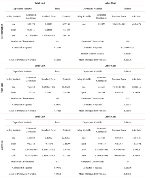
The results in Table 2 for the life-cycle stage after reconstruction indicate that the coefficient for the last year’s maintenance activities is positive. This observation is con-sistent with practice: more maintenance activities are reserved to be done at the time when a flush seal is performed. The maintenance cost between the reconstruction and flush seal can be viewed as constant over the years, because the coefficient for age is not significant.

The coefficient for elevation is positive, which makes sense because roads at higher elevations may have more chance of extreme weather as well as other road features that require maintenance (e.g., a guard rail). These observations also can be found in other maintenance cost components, including labor cost, equipment cost, and materials cost.

The results for the life-cycle stage Flush Seal indicates that only the variable representing the maintenance work when Chip Seal is performed is significant. This observation is consistent with practice, delaying maintenance work to be done when such a major preventive maintenance as Chip Seal is performed. This result also can be found in other maintenance cost components.

Table 2 shows the results for the life-cycle stage after Chip Seal, which ends at a re-construction. The results indicate that the coefficient for the “maintenance cost at the year of reconstruction” is negative because some maintenance activities may be saved to be done at the time of major construction work. The coefficient for road elevation is positive, which is reasonable because more potential maintenance work could be created when a road is at a high elevation. Examples of such potential maintenance work in-clude that for guard rails, slopes, and snow removal. Traffic has a positive coefficient, which is also consistent with expectations. These observations can be found in the re-sults for maintenance cost components.

Based on the results for these three life cycle stages, it can be seen that the mainten-ance costs in the years when construction, flush seal, and chip are performed signifi-cantly vary from those of other years. They cost more or less than the regular year, de-pending upon the nature of the maintenance work. Elevation is an important influen-cing factor to the maintenance costs. Traffic is another factor that plays a significant role. Age, however, does not show a significant impact on the maintenance cost.

5.4. Regression Models for the Roads in Prioritization Category 4

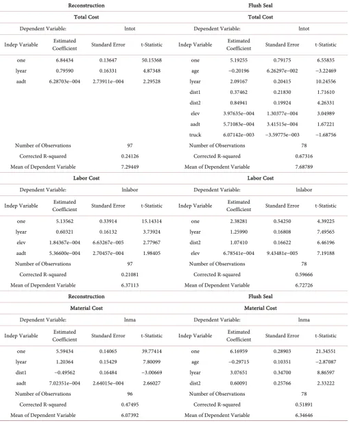
For Category 4, four linear regression models were developed, one for each life-cycle stage as shown in Figure 1: after reconstruction, after flush seal, after first chip seal, and after the second chip seal. Each life-cycle stage starts at the next year after the major maintenance activities, and ends at the end when these major maintenance activities are performed. The results of the model are presented in Table 3.

(11)

[image:11.595.47.551.89.715.2]

Table 2. Regression models for the roads in prioritization Category 3.

Re

co

ns

tr

uc

tio

n

Total Cost Labor Cost

Dependent Variable: lntot Dependent Variable: lnlabor

one 5.22175 0.60923 8.57101 one 6.22976 9.86522e−002 63.14873

lyear 0.76511 0.24410 3.13439

elev 2.61157e−004 1.27936e−004 2.04131

Corrected R-squared 0.12134 Corrected R-squared 0.00000e+000

Durbin-Watson Statistic 0.85384

Flu

sh

S

ea

l

one 7.23358 8.94882e−002 80.83270 one 6.36667 7.74854e−002 82.16616

lyear 1.35252 0.17832 7.58490 lyear 0.97188 0.15440 6.29458

C

hi

p S

eal

one 5.95503 0.46492 12.80873 one 5.37183 0.44704 12.01641

lyear 0.52712 −0.18476 −2.85306 lyear −0.48416 0.17765 −2.72532

elev 2.29486e−004 8.29841e−005 2.76542 elev 1.51135e−004 7.97929e−005 1.89409

aadt 5.97617e−004 1.41487e−004 4.22384 aadt 6.34517e−004 1.36046e−004 4.66399

(12)

Continued

Re

co

ns

tr

uc

tio

n

Material Cost Equipment Cost

Dependent Variable: lnma Dependent Variable: lneq

one 2.76351 0.80326 3.44035 one 3.23098 0.68499 4.71685

lyear 1.36009 0.32184 4.22592 elev 3.99350e−004 1.44481e−004 2.76404

elev 4.61092e−004 1.68682e−004 2.73351

Corrected R-squared 0.21176 Corrected R-squared 7.09088e−002

Flu

sh

S

ea

l

Indept Variable _CoefficientEstimated Standard Error t-Statistic Indep Variable _CoefficientEstimated Standard Error t-Statistic

one 5.46978 0.17230 31.74660 one 6.13286 0.19015 32.25351

lyear 1.81760 0.34332 5.29418 age −0.13997 7.10209e−002 −1.97088

lyear 1.07427 0.23502 4.57098

C

hi

p S

eal

one 4.13053 0.70597 5.85082 one 4.00296 0.52272 7.65788

age 0.11679 6.19514e−002 1.88524 lyear −0.63538 0.20773 −3.05871

lyear −0.87590 0.27677 −3.16474 elev 3.50827e−004 9.33017e−005 3.76014

elev 2.70935e−004 1.18212e−004 2.29195 aadt 5.96674e−004 1.59078e−004 3.75083

aadt 6.77556e−004 1.99749e−004 3.39203

(13)

[image:13.595.44.554.90.708.2]

Table 3. Linear regression models for the roads in prioritization Category 4.

Reconstruction Flush Seal

one 6.84434 0.13647 50.15368 one 5.19255 0.79175 6.55835

lyear 0.79590 0.16331 4.87348 age −0.20196 6.26297e−002 −3.22469

aadt 6.28703e−004 2.73911e−004 2.29528 lyear 2.09167 0.20415 10.24556

dist1 0.37462 0.21830 1.71610

dist2 0.84941 0.19924 4.26331

elev 3.97635e−004 1.30377e−004 3.04989 aadt 5.71083e−004 3.41515e−004 1.67221 truck 6.07142e−003 −3.59775e−003 −1.68756

one 5.13562 0.33914 15.14314 one 2.38281 0.54250 4.39225

lyear 0.60321 0.16132 3.73924 lyear 1.25990 0.16808 7.49565

elev 1.84367e−004 6.63267e−005 2.77967 dist2 1.07410 0.16622 6.46196

aadt 5.36600e−004 2.70457e−004 1.98405 elev 6.78541e−004 9.43481e−005 7.19188

Reconstruction Flush Seal

Material Cost Material Cost

one 5.59434 0.14065 39.77414 one 6.16959 0.28903 21.34551

lyear 1.20364 0.15429 7.80099 age −0.29715 0.10351 −2.87087

dist1 −0.49562 0.16484 −3.00669 lyear 3.07651 0.34700 8.86597

aadt 7.02351e−004 2.64015e−004 2.66027 dist2 0.60091 0.25766 2.33222

(14)

Continued

Equipment Equipment

one 5.76825 0.10346 55.75149 one 2.14434 0.76851 2.79024

lyear 0.51890 0.21725 2.38850 age −0.25160 7.70902e−002 −3.26374

lyear 1.53446 0.25827 5.94137

dist1 0.70683 0.28343 2.49387

dist2 1.20197 0.22563 5.32727

elev 6.91082e−004 1.40269e−004 4.92683

Corrected R-squared 4.67198e−002 Corrected R-squared 0.52516

Chip Seal-1 Chip Seal-2

one 6.91182 0.11215 61.63111 one 6.16464 0.61684 9.99388

lyear 1.81242 0.19820 9.14448 age 7.30700e−002 4.75945e−002 1.53526

dist1 0.31118 0.15951 1.95086 lyear −0.51297 0.21971 −2.33473

dist1 −0.35433 0.19684 −1.80010

elev 1.73129e−004 7.67915e−005 2.25453 aadt 1.51324e−003 7.35471e−004 2.05750 truck −1.29371e−002 6.05241e−003 −2.13752

one 5.64555 0.21227 26.59612 one 4.05502 0.47710 8.49922

lyear 1.29042 0.17225 7.49169 age 0.12064 4.42940e−002 2.72354

dist1 0.74466 0.23196 3.21034 lyear −0.65300 0.20709 −3.15322

dist2 0.63657 0.23240 2.73915 elev 2.91755e−004 6.84721e−005 4.26093

aadt 1.77472e−003 6.58573e−004 2.69479

(15)

Continued

Chip Seal-1 Chip Seal-2

Material Cost Material Cost

one 5.47692 0.13377 40.94294 one 5.70053 0.15453 36.88976

lyear 2.49629 0.29912 8.34551 dist1 −0.79064 0.23831 −3.31764

Equipment Equipment

one 5.48704 0.13220 41.50479 one 3.50169 0.57218 6.11988

lyear 1.33063 0.23364 5.69523 age 0.13717 5.31210e−002 2.58223

dist1 0.32468 0.18803 1.72669 lyear −0.76871 0.24836 −3.09514

elev 3.18557e−004 8.21175e−005 3.87929 aadt 1.34731e−003 7.89815e−004 1.70586

traffic flow, which is consistent with expectation. These findings also can be found in the models for the four cost components: labor, equipment, materials, and stockpile.

For the second life-cycle stage starting after flush seal is performed, relatively more variables are identified as significant to the maintenance cost. It can be seen that the va-riable representing the last year is significant, which is reasonable. Traffic flow is also significant. Age is significant, but with a negative coefficient. If the life-cycle span is short and many maintenance activities are frequently reserved for the last year, it is possible that the maintenance cost appears to decline with year; this has been con-firmed by respondents from some state DOT’s Maintenance Divisions as part of the survey conducted in this study.

(16)

expen-sive it is to maintain it; this is consistent with our expectations. These findings also can be found from the results for the four maintenance cost components.

The results for the third stage—starting from after a chip seal and ending at another chip seal—indicate that there are fewer significant variables. Whether or not a chip seal was performed in a year is important. The coefficient for the variable “last year”, which is the year with a chip seal was performed, is positive. This is reasonable. In this life- cycle stage, District 1 showed the most costly maintenance. This observation may be relevant regarding what type of equipment is used for the second chip seal in various districts; this is because the results for the four cost components indicate that the ma-terial costs between Districts 1 and 2 are the same, statistically.

The results for the last life cycle stage are very different from those for the first three segments. Age is significant. The total maintenance cost increased each year, which is understandable. The coefficient for the maintenance cost incurred in the last year is negative, which implies that the “last year” maintenance less expensive because other maintenance tasks were saved to be done during the reconstruction in this year. Among the three districts, District 1 has the least cost. This observation is relevant to mainten-ance practice, probably regarding the type of materials used in different districts. This result also can be found from the data for the four cost components. Traffic flow AADT is significant, which is consistent with expectations

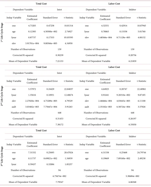
5.5. Regression Models for Roads in Prioritization Category 5

There is no clear definition in NDOT on the life cycle for routes in maintenance priori-tization Category 5. For simplicity, this study proposes three stages for the life cycle of a Category 5 route. The first stage starts after the completion of reconstruction, such as “2'' PBS with OG”, and ends at a flush seal or a chip seal. The second stage starts after a flush seal or a chip seal and ends at the completion of another flush seal or chip seal. The third stage starts after a flush or a chip seal, and ends at a construction. The second stage could be repeated many times; this is different from the life-cycle stages for Cate-gory 4, in which the middle stages are each performed one time only.

The results for the first life-cycle stage in Table 4 show that age, the last mainten-ance, and elevation are significant factors influencing the maintenance cost each year. It is a natural expectation that total maintenance cost increases with year, because declin-ing road conditions generate more maintenance work. The last year maintenance, which is either flush seal or chip seal, involves maintenance with more expensive mate-rials or equipment. The elevation at which a road is located influences maintenance cost. The higher elevation at which a road is located, the more expensive it is to main-tain. All these observations can be found in the models for the four maintenance cost components.

(17)

[image:17.595.47.553.87.714.2]

Table 4. Linear regression models for the roads in prioritization Category 5.

1

st L

ife C

yc

le S

ta

ge

one 4.73205 0.47258 10.01314 one 4.32551 0.42914 10.07945

age 0.12385 4.50500e−002 2.74927 lyear 0.78063 0.15558 5.01760

lyear 0.87737 0.17353 05.05593 elev 3.48566e−004 8.71128e−005 4.00132

elev 3.91701e−004 9.00566e−005 4.34950

2

nd L

ife C

yc

le S

ta

ge

one 5.57972 0.24429 22.84037 one 4.64925 0.20747 22.40961

lyear 1.35616 0.10931 12.40674 lyear 0.91641 9.28310e−002 9.87185

elev 2.27820e−004 4.75289e−005 4.79329 elev 2.46666e−004 4.03643e−005 6.11100

aadt 3.03482e−003 7.75647e−004 3.91263 aadt 2.35182e−003 6.58724e−004 3.57026

3

rd L

ife C

yc

le

St

ag

e

one 7.31532 0.25695 28.47024 one 6.31538 0.25468 24.79744

age 0.11737 8.69821e−002 1.34939 age 0.19669 7.89160e−002 2.49238

lyear 0.59437 0.32084 1.85257

Corrected R-squared 6.75674e−002 Corrected R-squared 5.30684e−002

(18)

Continued

1

st L

ife C

yc

le S

ta

ge

one 1.77701 0.86607 2.05181 one 2.45308 0.50058 4.90043

age 0.25317 8.25596e−002 3.06651 lyear 0.88297 0.18148 4.86544

lyear 1.22293 0.31802 3.84543 elev 6.22756e−004 1.01615e−004 6.12858

elev 5.75305e−004 1.65039e−004 3.48586

2

nd L

ife C

yc

le S

ta

ge

one 4.52583 0.18490 24.47656 one 4.29400 0.29732 14.44254

lyear 2.38705 0.18875 12.64682 age 0.10612 3.07889e−002 −−3.44663

aadt 5.12930e−003 1.33309e−003 3.84767 lyear 1.04501 0.13215 7.90795

elev 2.52489e−004 5.38903e−005 4.68523

aadt 2.04244e−003 8.90404e−004 2.29384

3

rd L

ife C

yc

le

St

ag

e

one 6.20010 0.14017 44.23313 one 6.31784 0.16710 37.80960

lyear 0.63605 0.27740 2.29287 lyear 0.78032 0.33069 2.35967

Corrected R-squared 4.37733e−002 Corrected R-squared 4.68188e−002

(19)

performed at different stages of road deterioration conditions. Traffic flow shows a positive impact. The results for the last life-cycle stage show that age and the last year maintenance (reconstruction) are significant factors. It is understandable that more maintenance is needed as roads age.

In the last year, when reconstructions were performed, some costs of these recon-structions were counted as maintenance equal to those for flush seals or chip seals. Thus, the last year maintenance becomes outstandingly expensive.

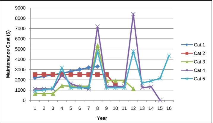
5.6. Annual Maintenance Costs for the Five Categories of Roads

[image:19.595.195.554.477.685.2]

The annual maintenance cost profiles for these five categories of roads are presented in

Figure 3. For an asphalt roadway section in Category 1, the elevation is assumed to be

2400 ft, and the AADT is 27,000; the total maintenance costs for an eight-year life cycle can be calculated using the function coefficients given in Table 1. As shown in Figure 3, the total costs increase with year. The annual maintenance cost in the eighth year becomes lower than the linear trend because of the reconstruction done that year. For a road section in Category 2 with an assumed average elevation 3987 ft and an average AADT of 11,786, the profile of annual maintenance costs can be calculated using the coefficients in Table 1. It can be seen from Figure 3 that the maintenance costs are constant, and would drop in the last year. Given the 12-year life cycle presented in

Fig-ure 1 for the roads in Category 3, a road section is assumed to have an average

eleva-tion of 4900 ft and an average AADT of 800; the annual maintenance profile can be calculated using the coefficients in Table 2. The profile displayed in Figure 3 indicates that the annual maintenance costs jump when flush seal and chip seal are performed that year, and drop when there is a reconstruction. The jump in maintenance cost caused by chip seal is more than that by flush seal. Within each life cycle, the annual maintenance costs are constant.

Figure 3. Comparison of annual maintenance cost profile for roads in five categories.

0 1000 2000 3000 4000 5000 6000 7000 8000 9000

1 2 3 4 5 6 7 8 9 10 11 12 13 14 15 16

M

ai

n

ten

an

ce C

o

st

(

$)

Year

Cat 1

Cat 2

Cat 3

Cat 4

(20)

For a road section in Category 4, the profile of the annual maintenance cost is calcu-lated using the values of the coefficients in Table 3. The road section is assumed to be located in District 1. Its elevation is 4700 ft, and it carries traffic with an AADT of 280. It can be seen from Figure 3 that the annual maintenance costs increase when there are flush seal and chip seals, and decrease when there is a reconstruction. The increase in cost with a flush seal is noticeably less than that with a chip seal. The first chip seal in-curs less cost than the second one. When producing the annual maintenance profile for Category 5, the values of the coefficients in Table 4 are used. It is assumed that a road section has elevation 5000 ft, and has an AADT of 130. It can be seen from Figure 3 that the annual maintenance costs increase significantly during such events as flush seals, chip seals, and construction.

It is clear that the annual maintenance costs for Categories 1 and 2 are higher than that for the other three categories. Major preventive or reconstruction activities signifi-cantly influence the maintenance cost, and have to be considered when calculating the annual maintenance costs.

6. Conclusions and Future Study Needs

6.1. Conclusions

In this study, linear regression models were developed to estimate annual maintenance costs for highway maintenance. Consistent with the maintenance road classification adopted by NDOT, five prioritization categories of roads were considered for model development. Categories 1 and 2 each included only one life-cycle stage, spanning eight and ten years, respectively. Categories 3 and 4 include three and four life-cycle stages, respectively; each stage is associated with certain maintenance activities and has three to four years duration. At NDOT, there was no specific definition on the life cycle for Category 5; therefore, three stages were defined in this study. For each stage of the life cycles in these five categories of roads, linear regression models were developed. In ad-dition to total maintenance cost, this study also developed linear regression models for four maintenance cost components: labor, equipment, materials, and stockpile.

Important influencing factors on annual maintenance costs were considered in this study: age of road, the type of maintenance activities in the last year of maintenance life cycle, elevation, district, and traffic. The results indicate that road age is a significant factor for some life cycle stages and some maintenance cost components. During the time period of a life-cycle stage, the annual maintenance cost may be kept the same. The maintenance activities in NDOT may have been scheduled by considering whether they are close to the time when a preventive maintenance or reconstruction is to be performed.

(21)

mainten-ance. Thus, they were singled out in the cost estimation of this study by using indicator variables. Roadways with high elevation tend to be constructed with special safety fea-tures, such as guard rails, which would produce high maintenance costs. This percep-tion was validated from the results of the models. Traffic flow deteriorates roads and generates the need for maintenance. Its impact on maintenance cost is also reflected in the model estimation results. Different districts may adopt different maintenance prac-tices in terms of the materials and equipment used in their districts; this was observed from the models developed in this study.

It can be seen that the developed models uniquely integrate the life-cycle concept of pavement by developing different models for different stages in the life cycles. These life-cycle stages also represent the conditions of a road section. The practice of main-tenance activities adopted in NDOT was fully considered in developing these models. The variables used in the models can be easily made available, and can provide the basis for the models to be incorporated into NDOT’s pavement management and mainten-ance management systems for estimating future maintenmainten-ance costs. NDOT could use these models to estimate the maintenance costs in order to submit cost requirements to the State of Nevada’s legislation.

6.2. Future Study Needs

Sampling is a major issue for developing the regression models for some categories of road like Categories 1 and 2. With samples covering more areas in Nevada, useful va-riables such as district can be used, by which more accurate estimation of annual main-tenance cost can be produced. The definition of life cycle influences the availability of sufficient samples. For example, the life cycle for Category 1 starts after a certain con-struction and ends at the same type of concon-struction. This life cycle may be hard to find in the database. Certain approximation was used in this study to extract the samples for Category 1. This sampling may need to be revisited when the model is adopted by NDOT.

Acknowledgements

The first author would like to thank Mr. Kent E. Mayer of the Nevada Department of Transportation who provided assistance in collecting the maintenance data.

References

[1] Anani, S.B. (2008) Revisiting the Estimation of Highway Maintenance Marginal Cost. Doc-toral Dissertation, Department of Civil and Environmental Engineering, University of Cal-ifornia, Berkeley.

[2] Gibby, R., Kitamura, R. and Zhao, H. (1990) Evaluation of Truck Impacts on Pavement Maintenance Costs. Transportation Research Record, 1262, 48-56.

[3] Hand, A.J. (1995) Development of Life-Cycle Cost Analysis Procedures for Nevada’s Flexi-ble Pavements. Master Thesis, Department of Civil Engineering, University of Nevada. [4] Sebaaly, P.E., Venukanthen, S., Siddharthan, R., Hand, R. and Epps, J. (2000) Development

(22)

Submit or recommend next manuscript to SCIRP and we will provide best service for you:

Accepting pre-submission inquiries through Email, Facebook, LinkedIn, Twitter, etc. A wide selection of journals (inclusive of 9 subjects, more than 200 journals)

Providing 24-hour high-quality service User-friendly online submission system Fair and swift peer-review system

Efficient typesetting and proofreading procedure

Display of the result of downloads and visits, as well as the number of cited articles Maximum dissemination of your research work

Submit your manuscript at: http://papersubmission.scirp.org/