http://www.scirp.org/journal/jtts ISSN Online: 2160-0481
ISSN Print: 2160-0473
Investigating the Existence of Second Order
Spatial Autocorrelation in Crash Frequency
across Adjacent Freeway Segments
Eneliko Mulokozi, Hualiang (Harry) Teng
Department of Civil and Environmental Engineering and Construction, Howard R. Hughes College of Engineering, University of Nevada, Las Vegas, NV, USA
Abstract
This study developed spatial Poisson model to incorporate spatial autocorrelation in crash frequency across contagious freeway segments. Spatial autocorrelation is the presence of spatial pattern in crash frequency over space due to geographic proximi-ty. Usually crash caused congestion on a freeway segment propagates upstream and creates chance of occurring secondary crashes. This phenomenon makes the crash frequency on the contiguous freeway segments correlated. This correlation makes the distributional assumption of independence of crash frequency invalid. The existence of spatial autocorrelation is investigated by using Conditional autoregressive models (CAR models). The models are set up in a Bayesian modeling framework, to include terms which help to identify and quantify residual spatial autocorrelation for neigh-boring observation units. Models which recognize the presence of spatial dependence help to obtain unbiased estimates of parameters quantifying safety levels since the effects of spatial autocorrelation are accounted for in the modeling process. Based on CAR models, approximately 51% of crash frequencies across contiguous freeway segments are spatially auto-correlated. The incident rate ratios revealed that wider shoulder and weaving segments decreased crash frequency by factors of 0.84 and 0.75 respectively. The marginal impacts graphs showed that an increase in longitudinal space for segments with two lanes decreased crash frequency. However, an increase of facility width above three lanes results in more crashes, which indicates an in-crease in traffic flows and driving behavior leading to crashes. These results call an important step of analyzing contagious freeway segments simultaneously to account for the existence of spatial autocorrelation.
Keywords
Freeway Segments, Spatial Autocorrelation, Conditional Autoregressive Model,
How to cite this paper: Mulokozi, E. and Teng, H.L. (2016) Investigating the Exis-tence of Second Order Spatial Autocorrela-tion in Crash Frequency across Adjacent Freeway Segments. Journal of Transportation Technologies, 6, 286-296.
http://dx.doi.org/10.4236/jtts.2016.65026
Received: February 23, 2016 Accepted: September 25, 2016 Published: September 28, 2016
Copyright © 2016 by authors and Scientific Research Publishing Inc. This work is licensed under the Creative Commons Attribution International License (CC BY 4.0).
MCMC Simulation
1. Introduction
Crash frequency for contiguous roadway segments tends to be correlated because con-gestion caused by a crash on a segment propagates to upstream. The propagation could reach to upstream segment quickly if the crash is severe, the segment where the crash occurs is short and traffic entering the downstream is high. The congestion reached to upstream may cause secondary crashes, which makes the crash frequencies on the con-tiguous segments correlated. Usually crash frequency is modeled by a Poisson model (Noland et al., 2004 [1]; Quddus, 2008 [2] and Li et al., 2007 [3]) which includes a set of influencing factors such as geometric elements of the freeways, traffic characteristics, environmental factors, and human factors. The correlation of crash frequency on con-tiguous freeway segments cannot be taken account in such a Poisson regression model in previous study.
To deal with the correlation of crash frequency, the Poisson regression model is inte-grated with a Conditional Autoregressive Model (CAR) (Aguero-Valverde, 2013 [4] and 2014 [5]) where the spatial effects leading to residual autocorrelation in the crash fre-quency can be specified. CAR models contain a precision matrix to control the spatial autocorrelation structure of the random effects based on the weight matrix. Contiguity of freeway segments can be specified in the model by a binary coding where a code equals to 1 if the freeway segments share a common border and is zero otherwise. A spatial autocorrelation parameter with variance is used to indicate the amount of auto-correlation in the crash frequency. The Poisson model integrated with CAR model can be estimated in a Bayesian framework. Under this framework, the unknown para-meters are set to reflect prior knowledge. Posterior means can be derived based on Markov Chain Monte Carlo (MCMC) simulation using Gibbs and Metropolis steps as sampling techniques. This study developed a statistical model that can incorporate spa-tial autocorrelation on contiguous freeway segments. Crash data and related influen-cing factor data were collected from the freeways in the Las Vegas area of Nevada. The spatial models are calibrated and interpreted, which shows significant different obser-vations than those from using the traditional methods.
The remaining part of the paper is organized as follows. The first section presents review of previous work on addressing spatial effects of transportation measures. In the second section, the spatial Poisson model is described with the presentation of the estimation me-thod. The third section provides the description of data collection, which is followed by ca-librating the spatial Poisson models in the fourth section. Comparison between the non- spatial and spatial Poisson regression models is also included in the fourth section. The last section includes the conclusions and recommendations for future study needs.
2. Review of Previous Work
crash prediction models help to explain variability observed in crash frequency and avoid making inference on biased estimates. Black et al., 1998 [6] employed a network autocorrelation analysis to examine accidents distributed along the segments of a high-way system and found a significant level of positive spatial autocorrelation. El-Basyouny et al., 2009 [7] used Gaussian conditional autoregressive and multiple membership models on 281 urban segments in Vancouver, Canada and found that spatial autocor-relation across urban segments explained approximately 87.6% of the variability in crash rates for CAR model while it was approximately 98.5% for multiple member ship models. In addition to these findings, it was also revealed that AADT, business land use, number of lanes between signals and density of unsignalized intersections had sig-nificant positive impact on the number of crashes.
Guo et al. (2010) [8] employed Bayesian count and Gaussian models to incorporate corridor-level and intersection proximity spatial autocorrelations in predicting crash rate and crash frequency. It was revealed that the size of an intersection, traffic condi-tions for both through and turning movements and the coordination of signal phase have significant impacts on intersection safety. This implies that closeness of coordi-nated intersections is likely to stimulate differential driving behavior compared to iso-lated intersections.
Arthur R. M. [9] identified the existence of spatial autocorrelation based on Moran’s I statistics applied on neighboring network intersections. To be able to apply the con-cepts of spatial autocorrelation on intersections as opposed to network roadway seg-ments, the analysis considered the roadways as links and the intersections and the ad-justed frequencies of collisions as areas. The Moran’s I statistics values indicated the existence of clusters of collision frequencies while graphing these values identified a temporal fluctuation that follows a diurnal pattern which indicates clustering patterns. It was also revealed that daytime pattern suggests a high frequency of collisions on ma-jor arteries during the day, especially over rush hour where it would be reasonable to assume a more clustered pattern.
Wang et al. (2013) [10] used Poisson-based multivariate conditional autoregressive (CAR) models estimated by Bayesian Markov Chain Monte Carlo methods to examine the relationship between pedestrian crash counts across tracts areas and various attributes characterizing the network, land use and demography. The results indicated the tence of positive spatial autocorrelation across neighborhoods as a result of the exis-tence of latent heterogeneity or missing variables that trend in space which are likely to generate spatial clustering of crash counts. In addition to spatial autocorrelation identi-fication, their results also showed that there is a greater association of residences and commercial land uses with pedestrian crash risk across different severity levels due to high potential conflicts between pedestrian and vehicle movements.
on their relative risk levels. The results showed that including spatial effects compo-nents in modeling processes improved the overall goodness-of-fit performance of the model and affected the ranking results for site improvements. The results further re-vealed that including CAR model in modeling process accounts for the degree of over dispersion.
3. Model Specification and Estimation
Bayesian Hierarchical Model for Crash Frequency
Let yi denote the number of crashes observed in a freeway segment for the ith covariate pattern. Let the expected value of yi depend on the explanatory variables xi. The Poisson generalized linear model (Guo et al., 2010 [8]) with the natural link function in the lo-garithmic function can be specified as:
( )
i i , 1, ,ln µ =x′β i= n. (1)
i
µ denotes the expected value of the crash frequency for segment i, xi′ is the
ma-trix of observed influencing factors including an intercept, and
β
is the matrix ofre-gression coefficients which quantifies the impact of covariates on the expected crash frequency. Equation (1) can be used to model spatial pattern in the crash frequency across freeway segments via a matrix of the covariates which in this case are the geome-tric and traffic characteristics observed on the freeways. However, the observed crash frequency for Poisson model exhibit over-dispersion and to capture this effect we ex-tend equation 1 to include random effects, ∅i to account for the possible effects of
over-dispersion:
( )
ln µi =xi′β+ ∅ =i,i 1,,n. (2)
Under Bayesian modeling frame work, prior distributions for the unknown parame-ters are set to reflect prior knowledge about the parameparame-ters of interest (El-Basyouny et al., 2009 [7]; Guo et al., 2010 [8]; Aguero-Valverde and Jovanis, 2006 [12]; Bailey et al., 1995 [13]). In this case we assume an independent Gaussian prior (diffuse normal priors) for each regression coefficient, βjN m
(
j,νj)
with mean, mj equals 0 and variance,j
ν necessarily large. We also assume uniform priors for random effects,
( )
2 0,i U
σ
∅
where 2
(
)
0,U Mσ
σ with large variance, Mσ .
We further assume the existence of second order spatial effects (Bolstad, 2005 [14] and Gelman et al., 2014 [15]) unaccounted for by the covariates and specify a Condi-tional Autoregressive Priors (Lee, 2011 [16] and Kery, 2010 [17]):
2 1 1 1 , 1 1 n ki i i
k k n n
ki ki
i i
w N
w p w
ρ τ
ρ ρ ρ
= − = = ∅ ∅ ∅ + − + −
∑
∑
∑
. (3)
bor-der and is zero otherwise.
ρ
is a spatial autocorrelation parameter with variance equals 2τ . A statistically significant value of
ρ
away from 0 implies the existence of spatial autocorrelation of crash frequency for contiguous freeway segments. Bothρ
and itsvariance parameter, τ2 have an independent prior specified as follows:
Spatial autocorrelation: ρU 0,1
( )
; τ2 0,U(
Mτ)
. (4)Our decision to adopt Equation (3) is based on the appealing fact that (Kery, 2010 [17]) conducted a comparative research and identified that the random effects modeled by a conditional autoregressive (CAR) prior distribution specified by Equation (3) is the best because it produces consistently good results across the range of spatial lation scenarios considered. It also represents a range of strong and weak spatial corre-lation structures with a single set of random effects which is beyond the models pro-posed.
Inference for the above models is based on Markov Chain Monte Carlo (MCMC) simulation (Lee, 2011 [16]; Kery, 2010 [17] and Dobson, 2010 [18]) using a combination of sampling techniques. The variance parameters are Gibbs sampled from their full conditional truncated inverse gamma distributions, while the remaining parameters are updated using Metropolis steps. An important key part of the analysis based on sam-pling techniques is to be able to make valid inferences. This is possible by monitoring Markov chain convergence to the target densities. To ensure the Markov chain lies within the stable area of high likelihood we apply a burn-in of 20,000 samples to ensure that the samples drawn from the chains approximate the posterior distribution. We also apply a thinning equal to 10, to reduce autocorrelation of neighboring samples (Dobson, 2010 [18]). We monitor our results of convergence and stable posterior distributions based on trace plots and posterior densities of covariates. To estimate our models, we apply CARBayes package in an R software environment (Lee, 2014 [19]) and WINBUGS version 1.4.3 (Medical Research Council, 2015 [20]). Choosing the most parsimonious model is based on the Deviance information criterion (DIC), which is a generalization of Akaike Information Criterion (AIC) for Bayesian models. We also evaluate the signi-ficance of estimated parameters based on 95% credible intervals.
4. Data and Descriptive Statistics
This section requires dataset with a structure focusing on the investigation of a special case of unobserved heterogeneity: spatial dependence of crash frequency for contiguous freeway segments. The model inputs are traffic and geometric characteristics from con-tiguous freeway segments extracted from loop detectors managed by FAST. Freeway segments which shares a common border identified as natural delineation between en-trance and exit were considered. Since the purpose is to identify the existence of spatial dependence, contiguous freeway segments with missing traffic characteristics were re-moved from the study and retained only segments with all information required.
aid from a base map as a tracing tool. Furthermore, sensor codes with their locations were observed from Google maps and matched with the created GIS shapefile of free-way segments and traffic characteristics which included vehicular speed and traffic vo-lumes were extracted for each sensor located on those segments.
Geometric characteristics were obtained by changing a GIS shapefile to KMZ and overlay the resulting KMZ file on Google earth map for visual aid. Number of lanes, median shoulder and right shoulder were observed and measured from the overlaid KMZ file as shown on Table 1 which shows summarized data.
From Table 1, it is evident that there is a high variability of crash counts and an in-dication of the presence of over-dispersion since the standard deviation of the crash counts is greater compared to its mean. Geometric characteristics are also diverse as shown by the minimum and maximum values in addition to their mean and standard deviations. However, less can be learnt concerning the existence of spatial effects and our detailed discussion is focused on the results section which follows.
5. Model Results and Discussion
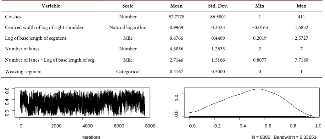
[image:6.595.196.554.481.707.2]CARBayes package version 4.0 and WINBUGS version 1.4.3 were used in estimating our models as shown on Table 2. To reduce autocorrelation of samples from the post-erior distribution, we thinned the sequence by keeping every 10th simulation draw from each sequence. We also discarded the first 20,000 samples and concentrate on the last 80,000 samples to be able to diminish the influences of early iterations and achieve the target distribution. This implies that our final results are summarized from 8,000 drawn samples. To ensure that the chain’s stationary distribution approximates the target distribution, we monitored our chain based on trace plots, historical plots of chain process as well as density plots of posterior means of the covariates and autocorrelation
Table 1. Estimated posterior means of covariates.
Covariates Estimates (95% credible interval)
Non-spatial GLM Poisson Spatial GLM Poisson model
Intercept 7.45 (6.78, 8.06) 4.46 (−3.69, 7.91)
Log (right shoulder) −1.08 (−1.25, −0.92) −0.17 (−1.63, 1.21)
Segment length in mile −8.03 (−8.10, −7.15) −4.21 (−8.16, 6.00)
No. of lanes −0.57 (−0.68, −0.45) −0.19 (−0.91, 1.25)
No. of lanes * seg. length 1.99 (1.80, 2.19) 1.18 (−1.20, 2.22)
Weaving segment −0.03 (−0.14, 0.07) −0.28 (−0.97, 0.48)
2
τ 1.22 (0.65, 2.89)
ρ 0.51 (0.09, 0.86)
term. Our final results include the trace plots for only the autocorrelation term as shown on Figure 1.
Based on the model fit criteria, the Spatial GLM Poisson model had a deviance In-formation criterion (DIC) equal to 243.8 which is small compared to a Non-spatial GLM model. This implies that the spatial model exhibited better fit to our data and therefore we interpret our results using the spatial GLM Poisson model. The final re-sults of a Spatial GLM Poisson model contain posterior means of covariates and auto-correlation term. The significance of these terms is based on 95% credible intervals. When the 95% credible intervals include zero, the corresponding factor is not signifi-cant at the 95% level and vice versa. We interpret our results based on the incident rate ratios which are exponentiated estimates and credible intervals as well as marginal im-pact for the interaction terms involving number of lanes and segment length.
Based on the results on Table 2, approximately 51% of crash frequencies across con-tiguous freeway segments are autocorrelated with a variance equals to 1.22. This results supports our aforementioned hypothesized situation that, there are spatial correlations of underlying processes generating crashes and these are likely to propagate across the adjacent segments. Most of the research activities analyze crash events on freeways based on the assumption that crash frequency observed on freeway segments are inde-pendent. This results lead to biased estimates if spatial effects are not included in our modeling processes.
[image:7.595.45.552.463.686.2]In addition to the aforementioned findings, we also investigated the impact of geo-metric elements on the crash frequency. The results are interpreted based on the expo-nentiated coefficients and credible intervals. As the results showed, right shoulder was found insignificant on individual bases. However, overall all variables were found
Table 2. Descriptive statistics for Bayesian spatial model.
Variable Scale Mean Std. Dev. Min Max
Crashes Number 57.7778 86.5801 1 411
Centred width of log of right shoulder Natural logarithm 0.9969 0.3323 −0.0163 1.6832
Log of base length of segment Mile 0.6766 0.4409 0.2019 2.5727
Number of lanes Number 4.3056 1.2833 2 7
Number of lanes * Log of base length of seg. Mile 2.7146 1.5166 0.8077 7.7180
Weaving segment Categorical 0.4167 0.5000 0 1
Figure 1. Posterior distribution of spatial correlation parameter.
0 2000 4000 6000 8000
0
.0
0
.4
0
.8
Iterations
0.0 0.2 0.4 0.6 0.8 1.0
0
.0
1
.0
[image:7.595.40.557.464.685.2]
to have an impact in the model. With these results it decreased crash frequency by a factor of 0.84 for segments with the same length and number of lanes and of the same type. This is reasonably true because wider shoulder provides enough space for drivers to maneuver to avoid crashes.
Weaving segments reduced crash frequency by a factor of 0.75 compared to non- weaving segments for segments with the same level of other influencing factors in-cluded in the model. This implies that drivers across these segments have time to make decisions to execute accelerations and decelerations activities to and from the freeway while still on the speed change lanes. In this case risk hazards to be encountered are likely to be avoided.
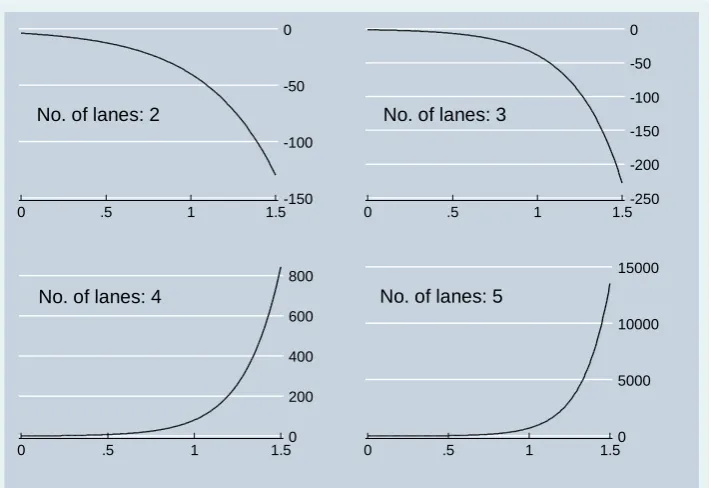
The impact of the number of lanes and segment lengths are better interpreted based on their marginal impacts as shown on Figure 2 including its corresponding margin-al effect function and in the context of longitudinmargin-al space and transverse space of the freeway facility. Including an interaction term is based on the fact that the influence of the extent longitudinal space depends on the transverse space available to accommo-date the number of vehicles available. As shown on Figure 2, as the longitudinal space increases for segments with two lanes, crash frequency decreased. This was also true for segments with three lanes. It should be understood that we interpret number of lanes as representing width of freeway in a transverse dimension.
(
)
(
)
.(
1.18* 4.21 exp 1.09 1.18*)
{
(
0.19 *)
}
.marginal eff
lanes length lanes
length
∂
= − −
∂
[image:8.595.197.553.426.670.2]However, when the width of freeway increases above three lanes, the facility experienced
Figure 2. Marginal effects on crash frequency.
No. of lanes: 2
-150 -100 -50 0
0 .5 1 1.5
No. of lanes: 3
-250 -200 -150 -100 -50 0
0 .5 1 1.5
No. of lanes: 4
0 200 400 600 800
0 .5 1 1.5
No. of lanes: 5
0 5000 10000 15000
0 .5 1 1.5
an increase in crash frequency. This can be explained by the fact that there are more traffic flows and driving activity associated with change lanes which is likely to stimu-late driver behavior as more vehicles occupy these segments. This is counter-intuitive when compared to the normal intuition indicated by two and three lanes as well as the previous research. The marginal effect graph also provides a clear picture of the inte-raction which could not be obvious based on the estimates alone.
6. Conclusions and Recommendation
Second order spatial effects are one of the components leading to unobserved hetero-geneity. If these effects are not included in quantifying the impacts of influencing fac-tors, the results obtained are likely to be biased. This study investigated the existence of second order spatial effects (spatial autocorrelation) for contiguous freeway segments. This is motivated by the fact that there are spatial correlations of underlying processes generating crashes and these are likely to propagate across the adjacent segments. Fur-thermore, there are interdependences across freeway characteristics in influencing crash occurrence which means the effect of one of the geometric elements depends on other geometric elements. Including interaction terms in modeling reduces the impact of unobserved heterogeneity because it accounts for effect modification resulting from modification variables.
Based on the aforementioned findings, it was found that wider shoulders and weav-ing segments reduced the level of crash frequency. Longitudinal space which was re-flected in the segment length exhibited differential impact across long freeway seg-ments. This differential impact can be explained by the existence of differential trans-verse space reflected in the number of travel lanes for long segments. This implies that interacting influencing factors helps to reduce the impact of unobserved modifiers leading to biasing results. It is imperative that safety modeling includes terms which explain any general or specific forms of unobserved heterogeneity. This helps to come up with actual impacts of the influencing factors retained in the model.
6.1. Model Application
The developed model can be applied as a discriminant model. This is based on the fact that spatial effects terms are included in the modeling process. Theories on the estima-tion process require integrating out these effects and summarize them in terms of va-riance, a method which leaves out the actual influence of the remaining factors. Based on Figure 2, a researcher can point out locations on the freeway network from which its factors exhibited more impacts on the crash frequency. For instance, with these re-sults segments with four and five lanes increased crash frequency compared to those with fewer number of lanes. These lanes require further investigation to be able to un-derstand causes of crash frequency occurrence.
reduce more crash frequency on freeways. For instance, our results for long segments with few numbers of lanes indicated that by increasing the longitudinal space we are able to reduce the number of crash frequency experienced. This is counter-intuiting with segments of the same length but have more lanes. This means we cannot adopt an alternative of increasing segment length on these locations. This helps to narrow down countermeasures alternatives and focus on Intelligent Transportation Systems designed for safety improvements on the freeway systems.
6.2. Future Research
The results from this study have indicated the existence of spatial autocorrelation across contiguous freeway segments. This implies that segments with spatial proximity con-stitute traffic and geometric characteristics which influence crash occurrence in a simi-lar trend. This phenomenon violates the distribution assumption of Poisson process un-der which crash events occur. Future research may involve simultaneity treatment of freeway segments in analyzing safety effects of factors which are believed to influence crash occurrence. Simultaneity behavior of observation unit can be incorporated in safety analysis by using simultaneous equation models which are the special case of the general structural equation models. In addition to solving the aforementioned problem of distributional assumption, general unobserved heterogeneity terms can further be incorporated to account for random effects.
References
[1] Noland, R.B. and Quddus, M.A. (2004) A Spatially Disaggregate Analysis of Road Causali-ties in England. Accident Analysis and Prevention, 36, 973-984.
http://dx.doi.org/10.1016/j.aap.2003.11.001
[2] Quddus, M.A. (2008) Modeling Area-Wide Count Outcomes with Spatial Autocorrelation and Heterogeneity: An Analysis of London Crash Data. Accident Analysis and Prevention, 40, 1486-1497. http://dx.doi.org/10.1016/j.aap.2008.03.009
[3] Li, L., Zhu, L. and Sui, Z.D. (2007) A GIS-Based Bayesian Approach for Analyzing Spa-tial-Temporal Patterns of Intra-City Motor Vehicle Crashes. Journal of Transport Geogra-phy, 15, 274-285. http://dx.doi.org/10.1016/j.jtrangeo.2006.08.005
[4] Aguero-Valverde, J. (2013) Multivariate Spatial Models of Excess Crash Frequency at Area Level: Case of Costa Rica. Accident Analysis and Prevention, 59, 365-373.
http://dx.doi.org/10.1016/j.aap.2013.06.014
[5] Aguero-Valverde, J. (2014) Direct Spatial Correlation in Crash Frequency Models: Estima-tion of the Effective Range, Journal of Transportation Safety & Security, 6, 21-33.
http://dx.doi.org/10.1080/19439962.2013.799108
[6] Black, R.W. and Thomas, I. (1998) Accidents on Belgium’s Motorways: A Network Auto-correlation Analysis. Journal of Transport Geography, 6, 23-31.
http://dx.doi.org/10.1016/S0966-6923(97)00037-9
[7] El-Basyouny, K. and Sayed, T. (2009) Urban Arterial Accident Prediction Models with Spa-tial Effects. Transportation Research Record: Journal of the Transportation Research Board, 2102, 27-33. http://dx.doi.org/10.3141/2102-04
Corridor-Level Spatial Correlations. Accident Analysis and Prevention, 42, 84-92. http://dx.doi.org/10.1016/j.aap.2009.07.005
[9] Arthur, R.M. (2003) Spatial and Temporal Analysis of Traffic Collisions (Order No. NQ87017). Available from ProQuest Dissertations & Theses Full Text (305346803).
[10] Wang, Y. and Kockelman, K.M. (2013) A Poisson-Lognormal Condition-Autoregressive Model for Multivariate Spatial Analysis of Pedestrian Crash Counts across Neighborhoods. Accident Analysis and Prevention, 60, 71-84. http://dx.doi.org/10.1016/j.aap.2013.07.030 [11] Miaou, S. and Song, J.J. (2005) Bayesian Ranking of Sites for Engineering Safety
Improve-ments: Decision Parameter, Treatability Concept, Statistical Criterion, and Spatial Depen-dence. Accident Analysis and Prevention, 37, 699-720.
http://dx.doi.org/10.1016/j.aap.2005.03.012
[12] Aguero-Valverde, J. and Jovanis, P.P. (2006) Spatial Analysis of Fatal and Injury Crashes in Pennsylvania. Accident Analysis and Prevention, 38, 618-625.
http://dx.doi.org/10.1016/j.aap.2005.12.006
[13] Bailey, C.T. and Gatrell, C.A. (1995) Interactive Spatial Data Analysis. John Wiley & Sons, Inc., New York.
[14] Bolstad, P. (2005) GIS Fundamentals: A First Text on Geographic Information Systems. 2nd Edition, Eider Press, White Bear Lake, Minnesota.
[15] Gelman, A., Carlin, J.B., Stern, H, S., Dunson, D.B., Vehtari, A. and Rubin, D.B. (2014) Bayesian Data Analysis. 3rd Edition, Taylor & Francis Group, LLC, FL.
[16] Lee, D. (2011) A Comparison of Conditional Autoregressive Models Used in Bayesian Dis-ease Mapping. Spatial and Spatio-Temporal Epidemiology, 2, 79-89.
http://dx.doi.org/10.1016/j.sste.2011.03.001
[17] Kery, M. (2010) Introduction to WINBUGS for Ecologists: A Bayesian Approach to Regres-sion, ANOVA, Mixed Models and Related Analyses. Elsevier Inc., Switzerland.
[18] Dobson, A. (2002) An Introduction to Generalized Linear Models. 2nd Edition, Chapman & Hall/CRC, USA.
[19] Dobson, A.J. and Barnett, A.G. (2010) An Introduction to Generalized Linear Models. 3rd Edition, Taylor & Francis Group, LLC, FL.
[20] Medical Research Council, Biostatistics Unit. WINBUGS Version 1.4.3.
Submit or recommend next manuscript to SCIRP and we will provide best service for you:
Accepting pre-submission inquiries through Email, Facebook, LinkedIn, Twitter, etc. A wide selection of journals (inclusive of 9 subjects, more than 200 journals)
Providing 24-hour high-quality service User-friendly online submission system Fair and swift peer-review system
Efficient typesetting and proofreading procedure
Display of the result of downloads and visits, as well as the number of cited articles Maximum dissemination of your research work
Submit your manuscript at: http://papersubmission.scirp.org/