Demand-Weighted Completeness Prediction for a Knowledge Base
Andrew Hopkinson and Amit Gurdasani and Dave Palfrey and Arpit Mittal Amazon Research Cambridge
Cambridge, UK
{hopkia, amitgurd, dpalfrey, mitarpit}@amazon.co.uk
Abstract
In this paper we introduce the notion of Demand-Weighted Completeness, allowing estimation of the completeness of a knowledge base with respect to how it is used. Defin-ing an entity by its classes, we employ usage data to predict the distribution over relations for that entity. For example, instances of per-sonin a knowledge base may require a birth date, name and nationality to be considered complete. These predicted relation distribu-tions enable detection of important gaps in the knowledge base, and define the required facts for unseen entities. Such characterisation of the knowledge base can also quantify how us-age and completeness change over time. We demonstrate a method to measure Demand-Weighted Completeness, and show that a sim-ple neural network model performs well at this prediction task.
1 Introduction
Knowledge Bases (KBs) are widely used for representing information in a structured format. Such KBs, including Wikidata (Vrandeˇci´c and Kr¨otzsch,2014), Google Knowledge Vault (Dong et al.,2014), and YAGO (Suchanek et al.,2007), often store information as facts in the form of triples, consisting of two entities and a relation be-tween them. KBs have many applications in fields such as machine translation, information retrieval and question answering (Ferrucci,2012).
When considering a KB’s suitability for a task, primary considerations are the number of facts it contains (F¨arber et al.,2015), and the precision of those facts. One metric which is often overlooked iscompleteness. This can be defined as the propor-tion of facts about an entity that are present in the KB as compared to an ideal KB which has every
fact that can be known about that entity. For ex-ample, previous research (Suchanek et al., 2011; Min et al.,2013) has shown that between 69% and 99% of entities in popular KBs lack at least one relation that other entities in the same class have. As of 2016, Wikidata knows the father of only 2% of all people in the KB (Gal´arraga et al., 2017). Google found that 71% of people in Freebase have no known place of birth, and 75% have no known nationality (Dong et al.,2014).
Previous work has focused on a general con-cept of completeness, where all KB entities are ex-pected to be fully complete, independent of how the KB is used (Motro, 1989;Razniewski et al., 2016;Zaveri et al.,2013). This is a problem be-cause different use cases of a KB may have dif-ferent completeness requirements. For this work, we were interested in determining a KB’s com-pleteness with respect to its query usage, which we termDemand-Weighted Completeness. For ex-ample, a relation used 100 times per day is more important than one only used twice per day.
1.1 Problem specification
We define our task as follows:
‘Given an entity E in a KB, and query usage
data of the KB, predict the distribution of relations thatEmust have in order for 95% of queries about
Eto be answered successfully.’
1.2 Motivation
Demand-Weighted Completeness allows us to pre-dict both important missing relations for existing entities, and relations required for unseen entities. As a result we can target acquisition of sources to fill important KB gaps.
It is possible to be entirely reactive when
dressing gaps in KB data. Failing queries can be examined and missing fields marked for investiga-tion. However, this approach assumes that:
1. the same KB entity will be accessed again in future, making the data acquisition useful. This is far from guaranteed.
2. the KB already contains all entities needed. While this may hold for some use cases, the most useful KB’s today grow and change to reflect a changing world.
Both assumptions become unnecessary with an abstract representation of entities, allowing gen-eralization to predict usage. The appropriateness of the abstract representation can be measured by how well the model distinguishes different entity types, and how well the model predicts actual us-age for a set of entities, either known or unknown. Further, the Demand-Weighted Completeness of a KB with respect to a specific task can be used as a metric for system performance at that task. By identifying gaps in the KB, it allows targeting of specific improvements to achieve the greatest increase in completeness.
Our work is the first to consider KB complete-ness using the distribution of observed KB queries as a signal. This paper details a learning-based approach that predicts the required relation dis-tributions for both seen and unseen class signa-tures (Section 3), and shows that a neural net-work model can generalize relation distributions efficiently and accurately compared to a baseline frequency-based approach (Section6).
2 Related work
Previous work has studied the completeness of the individual properties or database tables over which queries are executed (Razniewski and Nutt,2011; Razniewski et al., 2015). This approach is suit-able for KBs or use cases where individual tsuit-ables, and individual rows in those tables, are all of equal importance to the KB, or are queried separately.
Completeness of KBs has also been measured based on the cardinality of properties. Gal´arraga et al.(2017) andMirza et al.(2016) estimated car-dinality for several relations with respect to indi-vidual entities, yielding targeted completeness in-formation for specific entities. This approach de-pends on the availability of relevant free text, and uses handcrafted regular expressions to extract the
barackObama:
person: 1
politician: 1 democrat: 1 republican: 0
[image:2.595.312.419.70.150.2]writer: 1
Figure 1: Class signature forbarackObama. Other en-tities with the same class membership will have the same signature.
information, which can be noisy and doesn’t scale to large numbers of relations.
The potential for metrics around completeness and dynamicity of a KB are explored in Zaveri et al. (2013), focusing on the task-independent idea of completeness, and the temporal currency, volatility and timeliness of the KB contents. While their concept of timeliness has some similari-ties to demand-weighted completeness in its task-specific ’data currency’, we focus more on how the demand varies over time, and how the complete-ness of the KB varies with respect to that change in demand.
3 Representing Entities
3.1 Class Distributions
The data for a single entity does not generalize on its own. In order to generalize from observed usage information to unseen entities and unseen usage, and smooth out outliers, we need to com-bine data from similar entities. Such combination requires a shared entity representation, allowing combination of similar entities while preventing their confusion with dissimilar entities.
For this work, an entity may be a member of multiple classes (or types). We aggregate us-age across multiple entities by abstracting to their classes. Membership of a class can be considered as a binary attribute for an entity, with the entity’s membership of all the classes considered in the analysis forming aclass signature.
For example, the entitybarackObamais a per-son,politician,democrat, andwriter, among other classes. He is not arepublican. Considering these five classes as our class space, the class signature forbarackObamawould look like Figure1.
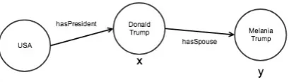
Figure 2: Graph representation of the facts needed to solve the query in Equation1. The path walked by the query can branch arbitrarily, but maintains a direction-ality from initial entities to result entities.
USA:
hasPresident: 13
hasCapital: 8
hasPopulation: 6 ...
Figure 3: Absolute usage data for the entityUSA.
class combinations not yet seen in the KB (though not entirely new classes).
3.2 Relation Distributions
KB queries can be considered as graph traversals, stepping through multiple edges of the knowl-edge graph to determine the result of multi-clause query. For example, the query:
y:hasPresident(USA, x)∧hasSpouse(y, x) (1)
determines the spouse of the president of the United States by composing two clauses, as shown in Figure2.
The demand-weighted importance of a relation
Rfor an entityEis defined as the number of query
clauses about E which contain R, as a fraction
of the total number of clauses about E. For ex-ample, Equation 1 contains two clauses. As the first clause queries for the hasPresident relation of the USA entity, we attribute this occurrence of hasPresident to the USA entity. Aggregating the clauses for an entity gives a total entity usage of the form seen in Figure3.
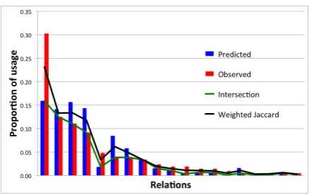
Since the distribution of relation usage is domi-nated by a few high-value relations (see Figure6), we only consider relations required to satisfy 95% of queries.
3.3 Predicting Relations from Classes
Combining the two representation methods above, we aim to predict the relation distribution for a
barackObama:
hasHeight: 0.16 hasBirthdate: 0.12 hasBirthplace: 0.08 hasSpouse: 0.07 hasChild: 0.05
Figure 4: An example of a predicted relation distribu-tion for an individual entity. The values represent the proportion of usage of the entity that requires the given relation.
given entity (as in Figure4) using the class mem-bership for the entity (as in Figure1). This pro-vides the expected usage profile of an entity, po-tentially before it has seen any usage.
4 Data and Models
4.1 Our knowledge base
We make use of a proprietary KB (Tunstall-Pedoe, 2010) constructed over several years, combining a hand-curated ontology with publicly available data from Wikipedia, Freebase, DBPedia, and other sources. However, the task can be applied to any KB with usage data, relations and classes. We use a subset of our KB for this analysis due to the limitation of model size as a function of the number of classes (input features) and the number of relations (output features).
Our usage data is generated by our Natural Lan-guage Understanding system, which produces KB queries from text utterances. Though it is difficult to remove all biases and errors from the system when operated at industrial scale, we use a hybrid system of curated rules and statistical methods to reduce such problems to a minimum. Such errors should not impact the way we evaluate different models for their ability to model the data itself.
4.2 Datasets
To create a class signature, we first determine the binary class membership vector for every entity in the usage dataset. We then group entities by class signature, so entities with identical class member-ship are grouped together.
Dataset Classes Relations Signatures
[image:4.595.307.526.59.197.2]D1small 4400 1300 12000 D2medium 8000 2000 25000 D3large 9400 2100 37000
Table 1: Dataset statistics.
person:
hasName: 31
hasAge: 18
hasHeight: 11 ...
Figure 5: Aggregated usage data for the classperson.
distribution of relations becomes. The data is di-vided into 10 cross-validation folds to ensure that no class signature appears in both the validation and training sets.
We generate 3 different sizes of dataset for ex-perimentation (see Table 1), to see how dataset size influences the models.
4.3 Relation prediction models 4.3.1 Baseline - Frequency-Based
In this approach, we compute the relation distri-bution for each individual class by summing the usage data for all entities of that class (see Section 3). This gives a combined raw relation usage as seen in Figure5.
For every class in the training set we store this raw relation distribution. At test time, we compute the predicted relation distribution for a class sig-nature as the normalized sum of the raw distribu-tions of all its classes. However, these single-class distributions do not capture the influence of class co-occurrence, where the presence of two classes together may have a stronger influence on the im-portance of a relation than each class on their own. Additionally, storing distributions for each class signature does not scale, and does not generalize to unseen class combinations.
4.3.2 Learning-Based Approaches
To investigate the impact of class co-occurrence, we use two different learning models to predict the relation distribution for a given set of input classes. The vector of classes comprising the class signa-ture is used as input to the learned models.
Linear regression. Using the normalized re-lation distribution for each class signature, we
Figure 6: Example histogram of the predicted (using a neural model) and observed relation distributions for a singleclass signature, showing the region of intersec-tion in green and the weighted Jaccard index in black.
trained a least-squares linear regression model to predict the relation distribution from a binary vec-tor of classes. This model has(n×m)parameters, wherenis the number of input classes andmis the
number of relations. We implemented our linear regression model using Scikit-learn toolkit ( Pe-dregosa et al.,2011).
Neural network. We trained a feed-forward neural network using the binary class vector as the input layer, with a low-dimensional (h) hidden
layer (with rectified linear unit as activation) fol-lowed by a softmax output layer of the size of the relation set. This model hash(n+m)parameters, which depending on the value ofhis significantly
smaller than the linear regression model. The ob-jective function used for training was Kullback-Liebler Divergence. We chose Keras (Chollet, 2015) to implement the neural network model. The model had a single 10-node Rectified Linear Unit hidden layer, with a softmax over the output.
5 Evaluation
We compare the predicted relation distributions to those observed for the test examples in two ways:
sig-nature. This is given by:
J = P
i
W(Ri)×Ri ∈(P∩O)
P
i
W(Ri)×Ri ∈(P∪O) (2)
whereP is the predicted distribution,Ois the ob-served distribution,W(Ri)is the mean weight of
relation Ri in P and O. We also calculate false
negatives (observed but not predicted) and false positives (predicted but not observed), by modify-ing the second term in the numerator of Equation 2to giveP\OandO\P, rather thanP∩O.
Intersection. We compute the intersection of the two distributions (see Figure6). This is a more strict comparison between the distributions which penalizes differences in weight for individual rela-tions. This is given by:
I =X
i
min(P(Ri), O(Ri)) (3)
5.1 Usage Weighted Evaluation
We also evaluated the models using the Weighted Jaccard index and Intersection methods, but weighting by usage counts for each signature. This metric rewards the models more for correctly predicting relation distributions for common class signatures in the usage data. While unweighted analysis is useful to examine how the model covers the breadth of the problem space, weighted evalu-ation more closely reflects the model’s utility for real usage data.
5.2 Temporal Prediction
Additionally, we evaluated the models on their ability to predict future usage. With an unchang-ing usage pattern, evaluation against future usage would be equivalent to cross-validation (assum-ing the same signature distribution in the folds). However, in many real world cases, usage of a KB varies over time, seasonally or as a result of chang-ing user requirements.
Therefore we also evaluated a neural model against future usage data to measure how elapsed time affected model performance. The datasets T1, T2, and T3 each contain 3 datasets (of simi-lar size to D1small, D2medium, and D1large), and
were created using usage data from time periods with a fixed offset,t. The base set was created at
timet0, T1 at timet0+t, T2 at timet0+ 2t, and
T3 at timet0+ 3t. A time interval was chosen that
reflected the known variability of the usage data,
Model Jaccard False Neg. False Pos.
D1small
Freq. 0.604 0.084 0.311
Regr. 0.522 0.102 0.376
NN 0.661 0.036 0.303
D2medium
Freq. 0.611 0.101 0.287
Regr. 0.557 0.084 0.358
NN 0.687 0.035 0.278
D3large
Freq. 0.616 0.105 0.278
Regr. 0.573 0.080 0.347
[image:5.595.308.525.65.279.2]NN 0.700 0.034 0.266
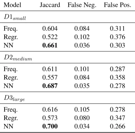
Table 2: Unweighted results for the three models on the three datasets.
such that we would expect the usage to not be the same.
6 Results
6.1 Cross-Validation
10-fold cross-validation results are shown in Ta-ble 2. The neural network model performs best, outperforming the baseline model by 6-8 per-centage points. The regression model performs worst, trailing the baseline model by 4-8 percent-age points.
6.1.1 Baseline
The baseline model shows little improvement with increasing amounts of data - the results from D1smallto D3large(3x more data points) only
im-prove by just over 1 percentage point. This sug-gests that this model is unable to generalise from the data, which is expected from the lack of class co-occurrence information in the model. Inter-estingly, the baseline model shows an increase in false negatives on the larger datasets, implying the lack of generalisation is more problematic for more fine-grained relation distributions.
6.1.2 Linear Regression
The linear regression model gives a much lower Jaccard measure than the baseline model. This is likely due to the number of parameters in the model relative to the number of examples. For D1small, the model has approximately 6m
under-determined system. For D3largethe number
of parameters rises to 20m, with 37k training ex-amples, maintaining the poor example:parameter ratio. From this we might expect the performance of the model to be invariant with the amount of data.
However, the larger datasets also have higher resolution relation distributions, as they are aggre-gated from more individual examples. This has the effect of reducing the impact of outliers in the data, giving improved predictions when the model gen-eralises. We do indeed see that the linear regres-sion model improves notably with larger datasets, closing the gap to the baseline model from 8 per-centage points to 4.
6.1.3 Neural Network
The neural network model shows much better per-formance than either of the other two methods. The Jaccard score is consistently 6-8% above the regression model, with far fewer false negatives and smaller numbers of false positives. This is likely to be due to the smaller number of param-eters of the neural model versus the linear regres-sion model. For D3large, the 10-node hidden layer
model amounts to 115k parameters with 37k train-ing examples, a far better ratio (though still not ideal) than for the linear regression model.
6.1.4 Weighted Evaluation
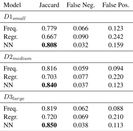
We include in Table 3 the results using the weighted evaluation scheme described in Sec-tion 5.1. This gives more usage-focused evalua-tion, emphasizing the non-uniform usage of dif-ferent class signatures. The D3large neural model
achieves 85% precision with a weighted evalua-tion. With the low rate of false negatives, this indi-cates that a similar model could be used to predict the necessary relations for KB usage.
6.2 Intersection
Table 4 gives measurements of the intersection metric. These show a similar trend to the Jac-card scores, with lower absolute values from the stricter evaluation metric. Although the Jaccard measure shows correct relation set prediction with a precision of 0.700, predicting the proportions for those relations accurately remains a difficult prob-lem. The best value we achieved was 0.398.
Model Jaccard False Neg. False Pos.
D1small
Freq. 0.779 0.066 0.123
Regr. 0.667 0.090 0.242
NN 0.808 0.032 0.159
D2medium
Freq. 0.816 0.059 0.094
Regr. 0.703 0.077 0.220
NN 0.840 0.037 0.123
D3large
Freq. 0.819 0.062 0.088
Regr. 0.720 0.069 0.210
[image:6.595.308.525.96.309.2]NN 0.850 0.038 0.113
Table 3: Usage-weighted results for the three models on the three datasets.
Model Freq. Regr. NN
Inter. 0.319 0.278 0.398
Table 4: Results for the three methods for the D3large dataset using the intersection metric. The difference between the methods is similar to the Jaccard measure above.
Interval T1 T2 T3
[image:6.595.341.492.411.449.2]D1small 0.661 0.659 0.657 D2medium 0.705 0.699 0.696 D3large 0.712 0.708 0.704
[image:6.595.331.500.573.639.2]6.3 Unweighted Temporal Prediction
In addition to evaluating models on their ability to predict the behaviour of unseen class signatures, we also evaluated the neural model on its ability to predict future usage behaviour. The results of this experiment are given in Table5.
We observe a very slight downward trend in the precision of the model using all three base datasets (D1small - D3large), with a steeper (but
still slight) downward trend for the larger datasets. This suggests that a model trained on usage data from one period of time will have significant pre-dictive power on future datasets.
7 Measuring Completeness of a KB
Once we have a suitable model of the expected re-lation distributions for class combinations, we use the model to predict the expected relation distribu-tion for specific entities in our KB. We then com-pare the predicted relation distribution to the ob-served relations for each specific entity. The com-pleteness of an entity is given by the sum of the relation proportions for the predicted relations the entity has in the KB.
Any gaps for an entity represent relations that, if added to the KB, would have a quantifiable pos-itive impact on the performance of the KB. By fo-cussing on the most important entities according to our usage, we can target fact addition to have the greatest impact to the usage the KB receives.
By aggregating the completeness values for a set of entities, we may estimate the completeness of subsets of the KB. This aggregation is weighted by the frequency with which the entity appears in the usage data, giving a usage-weighted measure of the subset’s completeness. These subsets can represent individual topics, individual classes of entity, or overall information about the KB as a whole.
For example, using the best neural model above on an unrepresentative subset of our KB, we evalu-ate the completeness of that subset at 58.3%. This not only implies that we are missing a substantial amount of necessary information for these entities with respect to the usage data chosen, but permits targeting of source acquisition to improve the en-tity completness in aggregate. For example, if we are missing a large number of hasBirthdatefacts for people, we might locate a source that has that information. We can quantify the benefit of that effort in terms of improved usage performance.
8 Conclusions and Future Work
We have introduced the notion of Demand-Weighted Completeness as a way of determining a KB’s suitability by employing usage data. We have demonstrated a method to predict the distri-bution of relations needed in a KB for entities of a given class signature, and have compared three different models for predicting these distributions. Further, we have described a method to measure the completeness of a KB using these distribu-tions.
For future work we would like to try com-plex neural network architectures, regularisation, and semantic embeddings or other abstracted re-lations to enhance the signatures. We would also like to investigate Good-Turing frequency estima-tion (Good,1953).
References
Franc¸ois Chollet. 2015. Keras. https://github.
com/fchollet/keras.
Xin Dong, Evgeniy Gabrilovich, Geremy Heitz, Wilko Horn, Ni Lao, Kevin Murphy, Thomas Strohmann, Shaohua Sun, and Wei Zhang. 2014. Knowledge Vault: A web-scale approach to probabilistic knowl-edge fusion. In Proceedings of the 20th ACM SIGKDD International Conference on Knowledge Discovery and Data Mining. ACM, New York, NY, USA, KDD ’14, pages 601–610. https://doi.
org/10.1145/2623330.2623623.
Michael F¨arber, Basil Ell, Carsten Menne, and Achim Rettinger. 2015. A comparative survey of DBpedia, Freebase, OpenCyc, Wikidata, and YAGO. Seman-tic Web Journal, July.
D. A. Ferrucci. 2012. Introduction to ”this is watson”. IBM J. Res. Dev.56(3):235–249. https://doi.
org/10.1147/JRD.2012.2184356.
Luis Gal´arraga, Simon Razniewski, Antoine Amarilli, and Fabian M. Suchanek. 2017. Predicting com-pleteness in knowledge bases. In Proceedings of the Tenth ACM International Conference on Web Search and Data Mining. ACM, New York, NY, USA, WSDM ’17, pages 375–383. https://
doi.org/10.1145/3018661.3018739.
I. J. Good. 1953. The population frequencies of species and the estimation of population parame-ters. Biometrika 40(3-4):237. https://doi.
org/10.1093/biomet/40.3-4.237.
Paul Jaccard. 1912. The distribution of the flora in the alpine zone.1. New Phytologist 11(2):37–50. https://doi.org/10.1111/
Bonan Min, Ralph Grishman, Li Wan, Chang Wang, and David Gondek. 2013. Distant supervision for relation extraction with an incomplete knowledge base. InHLT-NAACL. pages 777–782.
Paramita Mirza, Simon Razniewski, and Werner Nutt. 2016. Expanding Wikidata’s parenthood informa-tion by 178%, or how to mine relainforma-tion cardinali-ties. InISWC 2016 Posters & Demonstrations Trac. CEUR-WS. org.
Amihai Motro. 1989. Integrity = validity + com-pleteness. ACM Trans. Database Syst.14(4):480–
502. https://doi.org/10.1145/76902.
76904.
F. Pedregosa, G. Varoquaux, A. Gramfort, V. Michel, B. Thirion, O. Grisel, M. Blondel, P. Pretten-hofer, R. Weiss, V. Dubourg, J. Vanderplas, A. Pas-sos, D. Cournapeau, M. Brucher, M. Perrot, and E. Duchesnay. 2011. Scikit-learn: Machine learning in Python. Journal of Machine Learning Research 12:2825–2830.
Simon Razniewski, Flip Korn, Werner Nutt, and Di-vesh Srivastava. 2015. Identifying the extent of completeness of query answers over partially com-plete databases. In Proceedings of the 2015 ACM SIGMOD International Conference on Management of Data. ACM, New York, NY, USA, SIGMOD ’15, pages 561–576. https://doi.org/10.
1145/2723372.2750544.
Simon Razniewski and Werner Nutt. 2011. Complete-ness of queries over incomplete databases. VLDB 4:749–760.
Simon Razniewski, Fabian M Suchanek, and Werner Nutt. 2016. But what do we actually know. Pro-ceedings of AKBCpages 40–44.
Fabian Suchanek, David Gross-Amblard, and Serge Abiteboul. 2011. Watermarking for ontologies. The semantic web–ISWC 2011pages 697–713.
Fabian M. Suchanek, Gjergji Kasneci, and Gerhard Weikum. 2007. YAGO: A core of semantic knowl-edge. In Proceedings of the 16th International Conference on World Wide Web. ACM, New York, NY, USA, WWW ’07, pages 697–706. https:
//doi.org/10.1145/1242572.1242667.
William Tunstall-Pedoe. 2010. True Knowledge: Open-domain question answering using structured knowledge and inference. AI Magazine31(3):80–
92. https://doi.org/10.1609/aimag.
v31i3.2298.
Denny Vrandeˇci´c and Markus Kr¨otzsch. 2014. Wiki-data: A free collaborative knowledgebase. Com-mun. ACM 57(10):78–85. https://doi.org/
10.1145/2629489.