Applications of flexible querying to graph data

BIROn - Birkbeck Institutional Research Online

Poulovassilis, Alexandra (2018) Applications of flexible querying to graph

data. In: Fletcher, G. and Hidders, J. and Larriba-Pey, J.L. (eds.) Graph

Data Management: Fundamental Issues and Recent Developments.

Data-Centric Systems and Applications (DCSA). Springer, pp. 97-142. ISBN

9783319961927.

Downloaded from:

Usage Guidelines:

Please refer to usage guidelines at

or alternatively

Alexandra Poulovassilis

AbstractGraph data models provide flexibility and extensibility that makes them well-suited to modelling data that may be irregular, complex, and evolving in struc-ture and content. However, a consequence of this is that users may not be familiar with the full structure of the data, which itself may be changing over time, making it hard for users to formulate queries that precisely match the data graph and meet their information seeking requirements. There is a need therefore for flexible query-ing systems over graph data that can automatically make changes to the user’s query so as to find additional or different answers, and so help the user to retrieve informa-tion of relevance to them. This chapter describes recent work in this area, looking at a variety of graph query languages, applications, flexible querying techniques and implementations.

1 Introduction

Due to their fine modelling granularity (in its simplest form, comprising just nodes and edges, naturally representing entities and relationships), graph data models pro-vide flexibility and extensibility that is well-suited for modelling complex, dynami-cally evolving datasets. Moreover, graph data models are typidynami-cally semi-structured: there may not be a schema associated with the data; if there is a schema, then aspects of it may be missing from parts of the data and, conversely, parts of the data may not correspond to the schema. This makes graph data models well-suited to modelling heterogeneous and irregular datasets. Graph data models place a greater focus on the relationships between entities than other approaches to data modelling, viewing relationships as important as the entities themselves.

In recent years there has been a resurgence of academic and industry interest in graph databases, due to the generation of large volumes of data from web-based,

A.Poulovassilis

Birkbeck, University of London, Malet Street, London WC1E 7HX, e-mail: [email protected]

mobile and pervasive applications centered on the relationships between entities, for example: the web graph itself; RDF Linked Data1; social and collaboration net-works2 (Martin et al (2011); Suthers (2015)); transportation and communication networks (Deo (2004)); biological networks (Lacroix et al (2004); Leser and Trissl (2009)); workflows and business processes (Vanhatalo et al (2008)); customer re-lationship networks (Wu et al (2009)); intelligence networks (Ayers (1997); Chen et al (2011)); and much more!3

As the volume of graph-structured data continues to grow, users may not be aware of its full details and may need to be assisted by querying systems which do not re-quire queries to match exactly the data structures being queried, but rather can auto-matically make changes to the query so as to help the user find the information being sought. TheOPTIONALclause of SPARQL (Harris and Seaborne (2013)) has the aim of returning matchings to a query that may fail to match some of the query’s triple patterns. However, it is possible to “relax” a SPARQL query in ways other than just ignoring optional triple patterns, for example, making use of the knowledge encoded in an ontology associated with the data in order to replace an occurrence of a class in the query by a superclass, or an occurrence of a property by a superproperty.

This observation motivated the introduction in Hurtado et al (2008) of aRELAX clause for querying RDF data, which can be applied to those triple patterns of a query that the user would like to be matched flexibly. These triple patterns are suc-cessively made more general so that the overall query returns sucsuc-cessively more answers, at increasing “costs” from the exact form of the query. We review this work on ontology-based query relaxation in this section, starting with an example application in heterogeneous data integration in Section 1.1.

Section 2 goes beyond conjunctive queries to consider conjunctiveregular path

queriesover graph data, andapproximate answeringof such queries. In contrast to

query relaxation, which generally returns additional answers compared to the exact form of a database query, query approximation returns potentiallydifferentanswers to the exact form of a query.

Section 3 considers combining both query relaxation and approximate answering for conjunctive regular path queries over graph data, describing also an automaton-based implementation. Section 4 considers extending SPARQL 1.1 with query re-laxation and approximation, describing an implementation based on query rewrit-ing. Along the way, we consider applications of query relaxation and query approx-imation for graph data in areas such as heterogeneous data integration, ontology querying, educational networks, transport networks and analysis of user-system in-teractions. Section 5 covers additional topics: possible user interfaces for supporting users in incrementally constructing and understanding flexible queries and the an-swers being returned; and possible extensions to the query languages considered so far with additional flexibility beyond relaxation and approximation, and with ad-ditional expressivity in the form of path variables. Section 6 gives an overview of

1_{http://linkeddata.org, http://www.w3.org/standards/semanticweb, accessed at 18/6/2015} 2_{https://snap.stanford.edu/data, accessed at 18/6/2015}

related work on query languages for graph data and flexible querying of such data. Section 7 gives our concluding remarks and possible directions of future work.

Flexible Database Query Processing

Before begining our discussion of flexible query processing for graph data, we first review the main approaches to flexible query processing for other kinds of data. Due to the considerable breadth of this area, the references cited here are representative of the approaches discussed rather than an exhaustive list. Readers are referred to the proceedings of the biannual conference on Flexible Query Answering Systems (FQAS) for a broad coverage of work in this area.

Query languages for structured data models, such as SQL and OQL, include WHERE clauses that allow filtering criteria to be applied to the data matched by their SELECT clauses. Therefore a natural way to relax queries expressed in such languages is by dropping a selection criterion, or by ‘widening’ a selection criterion so as to match a broader range of values (Bosc and Pivert (1992); Heer et al (2008)). Another common approach to query relaxation is to allow fuzzymatching of se-lection criteria, accompanied by a scoring function that determines the degree of matching of the returned query answers (Galindo et al (1998); Na and Park (2005); Bordogna and Psaila (2008); Bosc et al (2009)). Conversely, queries can be made more specific by adding user preferences as additional filter conditions, with possi-bly fuzzy matching of such conditions (Mishra and Koudas (2009); Eckhardt et al (2011)). Chu et al (1996) use type abstraction hierarchies to both generalise and spe-cialise queries, while Zhou et al (2007) explore statistically-based query relaxation through ‘malleable’ schemas containing overlapping definitions of data structures and attributes.

Turning to approximate query answering, approaches include histograms (Ioan-nidis and Poosala (1999)), wavelets (Chakrabarti et al (2001)) and sampling (Bab-cock et al (2003)). Sassi et al (2012) describe a system that enables the user to issue an SQL aggregation query, see results as they are being produced, and dy-namically control query execution. Fink and Olteanu (2011) study approximation of conjunctive queries on probabilistic databases by specifying lower- and upper-bound queries that can be computed more efficiently.

In principle, techniques proposed for flexible querying of structured data can also be applied to graph-structured data. However, such techniques do not focus on the connections (i.e. edges and paths) inherent in graph-structured data, thus missing opportunities for further supporting the user through approximation or relaxation of the path structure that may be present in a graph query.

undertake query relaxation through removal of conditions from XPath expressions; Theobald et al (2005) support relaxation by expanding queries using vocabulary in-formation drawn from an ontology or thesaurus; Liu et al (2010) use available XML schemas to relax queries; and Hill et al (2010) use ontologies such as Wordnet to guide XML query relaxation. Buratti and Montesi (2008) discuss query approxi-mation for XML based on the notion of a cost-based edit distance for transforming one path into another within an XQuery expression, while Almendros-Jimenez et al (2014) propose a fuzzy approach to XPath query evaluation.

Similar approaches to those developed for XML can be adopted for flexible querying of graph-structured data, and indeed in subsequent sections of this chapter we discuss ontology-based relaxation of graph queries and also edit distance-based ranking of approximate answers to graph queries. However, the techniques proposed for flexibly querying XML generally assume one kind of relationship between en-tities (parent-child) whereas in graph-structured data there may be numerous rela-tionships, potentially giving rise to higher complexity and diversity in the data and requiring query approximation and relaxation techniques that are able to operate on the relationships referenced within a user’s query.

1.1 Example: Heterogeneous Data Integration

Much work has been done since the early 1990s in developing architectures and methodologies for integrating biological data (Goble and Stevens (2008)). Such in-tegrations are beneficial for scientists by providing them with easy access to more data, leading to more extensive and more reliable analyses and, ultimately, new sci-entific insights. Traditional data integration methodologies (Batini et al (1986)) re-quire semantic mappings between the different data sources to be initially deter-mined, so that a global integrated schema or ontology can be created through which the data in the sources can then be accessed. This approach means that significant resources for data integration projects must be committed up front, and an active area of research is how to reduce this up-front effort (Halevy et al (2006)). A gen-eral approach adopted is to present initially all of the source data in an unintegrated format, and to provide tools that allow data integrators to incrementally identify se-mantic relationships between the different data sources and incrementally improve the global schema. Such an approach is termed “pay-as-you-go” (Sarma and et al. (2008)), since the integration effort can be committed incrementally as time and resources allow.

dis-tributed queries posed over this (Siepen et al (2008))4. The development of the global schema took many months. An alternative approach would have been to adopt a “pay-as-you-go” integration approach, refining the global ontology by incremen-tally identifying common concepts between the data sources and integrating these using additional super-classes and super-properties.

For example, the initial ontology may include (amongst others) the classes

• Peptide1,Protein1,Peptide2,Protein2,Peptide3,Protein3,

arising from three source databases,DB1,DB2,DB3; for simplicity here, we assume that common concepts are commonly named, and we identify the data source re-lating to a concept by its subscript. Likewise, it may include (amongst others) the properties

• PepSeqi, 1≤i≤3, each with domainPeptideiand range Literal,

• Alignsi, 1≤i≤3, each with domainPeptideiand rangeProteini,

• AccessNoi, 1≤i≤3, each with domainProteiniand range Literal.

(In proteomics, proteins consist of several peptides, each peptide comprising a se-quence of amino acids; hence the properties PepSeqi above, in which the amino

acid sequence is represented as a Literal. In proteomics experiments, several pep-tides may result from a protein identification process and each peptide aligns against a set of proteins; hence the propertiesAlignsiabove. Each protein is characterized

by an Accession Number, c.f. the propertiesAccessNoiabove, a textual description,

its predicted mass, the organism in which it found, etc.).

A data integrator may observe some semantic alignments between the above classes and properties and may add the following superclasses and superproperties to the ontology in order to semantically integrate the underlying data extents from the three databases:

• superclassPeptideof classesPeptidei, 1≤i≤3

• superclassProteinof classesProteini, 1≤i≤3

• superpropertyPepSeqof propertiesPepSeqi, 1≤i≤3, with domainPeptideand

range Literal

• superpropertyAlignsof propertiesAlignsi, 1≤i≤3, with domainPeptideand

rangeProtein

• superpropertyAccessNoof propertiesAccessNoi, 1≤i≤3, with domainProtein

and range Literal.

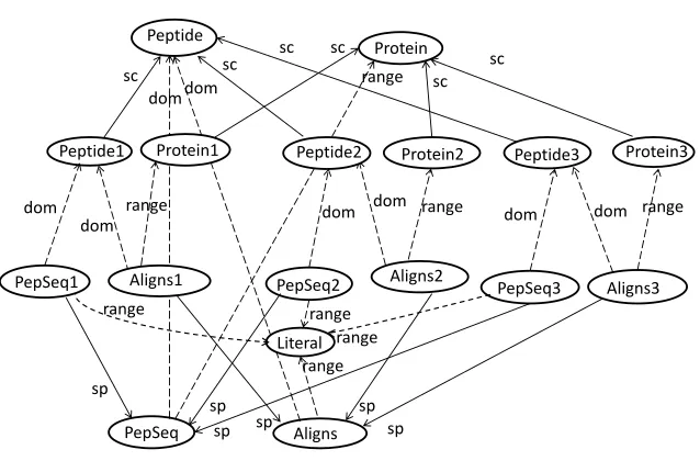
A fragment of this global ontology is shown in Figure 1 (omitting theAccessNoiand

AccessNoproperties, and the domain and range information ofPepSeqandAligns).

Consider now the following query posed over the global ontology by a user who is only familiar withDB1:

?Y, ?Z <- RELAX(?X,PepSeq1,"ATLITFLCDR"), RELAX(?X,Aligns1,?Y),

RELAX(?Y,AccessNo1,?Z)

Literal

Aligns PepSeq

sc sc

sc sc

sc sc

sp

sp sp sp

sp sp dom

dom dom

dom

dom dom

range range range

range _range

range range Literal dom

PepSeq1 Aligns1 _PepSeq2 Aligns2 _{PepSeq3 Aligns3}

Peptide1 Protein2 _Peptide3 Protein3

Peptide

Protein

Protein1 dom

Peptide2 range

Fig. 1 Example Ontology

The syntax used here is that of a conjunctive query comprising one or moretriple

patternson its right-hand side (RHS) — see Section 1.2, and zero or more

vari-ables on its left-hand side (LHS), which must also appear in the RHS. The entire RHS comprises agraph pattern— see Section 1.2. Variables are distinguished by an initial?. In its non-relaxed form, this query will return the identifiers and acces-sion numbers of proteins identified inDB1through experiments yielding the peptide sequence “ATLITFLCDR”.

A first level of relaxation of all three triple patterns in the above query results in the following query:

?Y, ?Z <- RELAX(?X,PepSeq,"ATLITFLCDR"), RELAX(?X,Aligns,?Y),

RELAX(?Y,AccessNo,?Z)

Evaluation of this query will expand the result set to include similar results also fromDB2andDB3, without the user needing to have detailed knowledge of their schemas.

1.2 Theoretical Foundations of Query Relaxation

Hurtado et al (2008) studied query relaxation in the setting of the RDF/S data model and showed that query relaxation can be naturally formalised usingRDFS entail-ment. The entailment was characterized by the derivation rules given in Figure 2, grounded in the semantics developed in Gutierrez et al (2004) and Hayes (2004), and encompassing a fragment of the overall set of RDFS entailment rules known as ρDF (Munoz et al (2007)).

In the setting of Hurtado et al (2008), anontology Kis a directed graph(NK,EK)

where each node inNK represents either a class or a property, soNK=classNodes

(NK)∪propertyNodes(NK); and each edge inEK is labelled with a symbol from

the set{sc,sp,dom,range}. These edge labels encompass a fragment of the RDFS vocabulary:rdfs:subClassOf,rdfs:subPropertyOf,rdfs:domain,rdfs:range, re-spectively.

In the accompanying data graphG= (N,E), each node inN represents an in-stance or a class and each edge inE a property. The intersection ofN andNK is

contained inclassNodes(NK). The predicatetype, representing the RDF vocabulary

rdf:type, can be used inE to connect an instance of a class to a node representing that class.

Pairwise disjoint setsU andL of URIs and literals are assumed, respectively. Also assumed is an infinite setV ofvariables, disjoint fromUandL. We abbreviate any union of the setsU,LandV by concatenating their names, e.g.U L=U∪L.

Nodes inNare labelled with constants fromU L(blank nodes are not considered in this work, and in any case their use is discouraged for Linked Data). Edges inE

are labelled either withtypeor a with symbol drawn from a finite alphabetΣsuch thattype∈/ΣandΣ∪ {type} ⊂U.

AnRDF triple is a tuplehs,p,oi ∈U×U×(U∪L), wheresis the subject, p

the predicate ando the object of the triple. A triple patternis a tuple hx,p,yi ∈

UV×UV×UV L. Agraph patternis a set of triple patterns. Given a triple patternt

(graph patternP),vars(t)(vars(P)) is the set of variables occurring in it.

AnRDF/S graph I= (NI,EI)is the union of an ontology graph K= (NK,EK)

and a data graphG= (N,E), i.e.NI=NK∪NandEI=EK∪E.

Subproperty (1)(a,sp,b)(b,sp,c) (a,sp,c) (2)

(a,sp,b)(x,a,y) (x,b,y)

Subclass (3) (a,sc,b)(b,sc,c) (a,sc,c) (4)

(a,sc,b)(x,type,a) (x,type,b)

Typing (5)(a,dom,c)(x,a,y) (x,type,c) (6)

(a,range,d)(x,a,y) (y,type,d)

Fig. 2 RDFS inference rules

Theclosure of an RDF/S graphI under these rules is denoted bycl(I). Given an RDF/S graph I, query evaluation takes place on the graph given by restrict-ingcl(I)to nodes inN∪classNodes(NK)and edges with labels in Σ∪ {type} ∪

propertyNodes(NK). Each such edge is viewed as an RDF triple for the purposes of

query evaluation.

In order to apply relaxation to queries, the subgraphs of the ontologyKinduced by edges labelledscandspneed to beacyclic, so that an unambiguous cost can be assigned to a relaxed query. Moreover,Kmust be equal to itsextended reduction,

extRed(K), which is computed as follows:

(a) computecl(K);

(b)apply the rules of Figure 3 in reverse until no more rules can be applied (applying a rule in reverse means deleting a triple deducible by the rule);

(c) apply rules 1 and 3 of Figure 2 in reverse until no more rules can be applied.

Requring thatK=extRed(K)allowsdirect relaxationsto be applied to queries (see below), which correspond to the “smallest” possible relaxation steps. This in turn allows an unambiguous cost to be associated with relaxed queries, so that query an-swers can be returned to users incrementally in order of increasing cost (see Hurtado et al (2008) for a detailed discussion).

(e1) (b,dom,c)(a,sp,b) (a,dom,c) (e2)

(b,range,c)(a,sp,b) (a,range,c)

(e3)(a,dom,b)(b,sc,c) (a,dom,c) (e4)

(a,range,b)(b,sc,c) (a,range,c)

Fig. 3 Additional rules for computing the extended reduction of an ontology

Following the terminology of Hurtado et al (2008), a triple pattern hx,p,yi

directly relaxes to a triple pattern hx0,p0,y0i with respect to an ontology K =

extRed(K), denoted hx,p,yi ≺ hx0,p0,y0i, ifvars(hx,p,yi) =vars(hx0,p0,y0i)and hx0,p0,y0iis derived fromhx,p,yiby applying some rulei, 1≤i≤6, from Figure 2. A triple patternhx,p,yirelaxes toa triple patternhx0,p0,y0i, denotedhx,p,yi ≤ hx0,p0,y0i, if there is a sequence of direct relaxations that deriveshx0,p0,y0i from hx,p,yi. Therelaxation cost of deriving hx0,p0,y0i fromhx,p,yiis the minimum cost of applying such a sequence of direct relaxations.

An essential aspect of this approach, which distinguishes it from earlier work on query relaxation, is that the answers to a query are ranked based on how ‘closely’ they satisfy the query. The notion of ranking is based on a structure called the

relax-ation graph, in which relaxed versions of the original query are ordered from less to

more general.

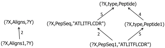
To illustrate, Figure 4 shows the relaxation graphs of two triple patterns: (?X,Aligns1,?Y)and(?X,PepSeq1,"ATLITFLCDR")

(?X,Aligns1,?Y) _{(?X,PepSeq1,"ATLITFLCDR")} (?X,PepSeq,"ATLITFLCDR") (?X,type,Peptide1)

(?X,type,Peptide)

(?X,Aligns,?Y)

2 _{2 5}

5 4

Fig. 4 Triple pattern relaxation graphs

Triple pattern relaxation is generalised to graph pattern relaxation using the notion of the direct productof partial orders. Thedirect product of n partial or-dersα1,α2, . . .αn, denotedα1⊗α2⊗. . .⊗αn, is another partial orderα such that

(a1, . . .an)α (b1, . . .bn)if and only ifaiαibifor all 1≤i≤n.

Consider graph patterns consisting ofntriple patterns,t1, . . . ,tn. The graph

pat-tern relaxation relation≤nis defined as≤ ⊗ ≤. . .⊗ ≤(ntimes). The direct graph

pattern relaxation relation ≺n is the reflexive and transitive reduction of ≤n. The

relaxation graphof a graph pattern is the directed acyclic graph induced by≺n.

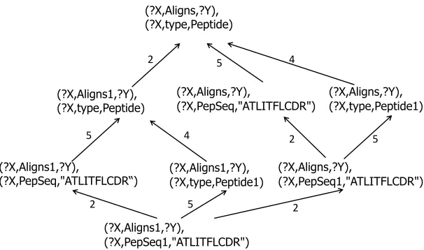
As an example, consider the graph pattern

(?X,Aligns1,?Y),(?X,PepSeq1,"ATLITFLCDR")

Figure 4 shows the relaxation graphs of its two triple patterns and Figure 5 shows their direct product.

Algorithm RelaxEval in Figure 6 (from Hurtado et al (2008)) incrementally computes the relaxed answer to a queryQand returns the answers in ranked order, where:maxLevelis the maximum number of relaxations desired for the evaluation of

Q;body(Q)denotes the graph pattern in the RHS ofQ; and the setdeltaFind(t0i,I)

consists of the tripleshs,p,oi ∈Isuch thatt0imatcheshs,p,oiand no triple pattern

directly belowt0iin the relaxation graph oftimatcheshs,p,oi. This algorithm

(?X,Aligns1,?Y),

(?X,PepSeq1,"ATLITFLCDR") (?X,Aligns1,?Y),

(?X,PepSeq,"ATLITFLCDR“) (?X,Aligns1,?Y),(?X,type,Peptide1)

(?X,Aligns,?Y),

(?X,PepSeq1,"ATLITFLCDR") (?X,Aligns,?Y),

(?X,PepSeq,"ATLITFLCDR") (?X,Aligns,?Y),

(?X,type,Peptide)

(?X,Aligns1,?Y), (?X,type,Peptide)

(?X,Aligns,?Y), (?X,type,Peptide1)

2

2

5

5

2 2

5

5

4

4

Fig. 5 Graph pattern relaxation graph

AlgorithmRelaxEval

Input:a queryQ, wherebody(Q) ={t1, . . . ,tn}; an RDF/S graphI; and an integermaxLevel.

Output:the set of ranked answer tuples.

1. k:=0,stillMore:=true

2. For eachti∈body(Q), compute the relaxation graphRioftiup to levelmaxLevel.

3. While (k≤maxLevelandstillMore) do

a. For each combination t01 ∈R1, . . . ,t0n ∈Rn such that ∑ilevel(t0i,Ri) =k do output

πH(deltaFind(t01,I)no. . .ondeltaFind(t0n,I))

b. k:=k+1

c. stillMore:=exist nodest01∈R1, . . . ,t0n∈Rnsuch that∑ilevel(t0i,Ri) =k

Fig. 6 Algorithm to compute the relaxed answer of a query

2 Beyond Conjunctive Queries : Regular Path Queries

Regular path querieshave been proposed by several researchers as a means of

as-sisting users in querying complex or irregular graph data by findingpathsthrough the data graph that match a given regular expression over edge labels (Cruz et al (1987); Mendelzon and Wood (1989, 1995); Fernandez and Suciu (1998)).

Consider the same simple data model as introduced above, comprising a directed graphG= (N,E), where each node inNis labelled with a constant and each edge in

Eis labelled with a symbol drawn from a finite alphabetΣ∪ {type}. Edges can be traversed both from their source to their target node and in reverse, from their target to their source node. Theinverseof an edge labell, denoted byl−, is used to specify the reverse traversal of an edge. LetΣ−={l−|l∈Σ}. Ifl∈Σ∪Σ−∪{type,type−}, we usel−to mean theinverseofl, that is, iflisafor somea∈Σ∪ {type}, thenl−

isa−, while iflisa−for somea∈Σ∪ {type}, thenl−isa.

Aregular path query(RPQ) Q has the form

vars←(X,R,Y) (1)

whereXandY are constants or variables,Ris a regular expression overΣ∪ {type}, andvars is the subset of {X,Y} that are variables. Aregular expression R over

Σ∪ {type}is defined as follows:

R:=ε|a|a−| |(R1·R2)|(R1|R2)|R∗|R+

whereεis the empty string,ais any symbol inΣ∪ {type}, “ ” denotes the disjunc-tion of all constants inΣ∪ {type}, and the operators have their usual meaning.

Asemipath(Calvanese et al (2000))pinG= (N,E)fromv∈N tow∈N is a

sequence of the form(v1,l1,v2,l2,v3, . . . ,vn,ln,vn+1), wheren≥0,v1=v,vn+1=w

and for eachvi,li,vi+1eithervi li

→vi+1∈Eorvi+1

l_i−

→vi∈E. A semipathp conforms

to a regular expressionRifl1· · ·ln∈L(R), the language denoted byR.

Given a RPQQand graphG, letθbe a matching from{X,Y}to nodes ofGthat maps each constant to itself and such that there is a semipath fromθ(X)toθ(Y) whose concatenation of edge labels is inL(R). TheanswerofQonGis the set of tuplesθ(vars)for all such matchingsθ.

Aconjunctive regular path query(CRPQ)Qconsisting ofnconjuncts has the

form

Z1, . . . ,Zm←(X1,R1,Y1), . . . ,(Xn,Rn,Yn) (2)

in which eachXiandYi, 1≤i≤n, is a variable or constant, eachZi, 1≤i≤m, is a

variable appearing in the body ofQ, and eachRi, 1≤i≤n, is a regular expression

overΣ∪ {type}.

semipath fromθ(Xi)toθ(Yi)that conforms toRi, for all 1≤i≤n. Theanswerof QonGis the set ofm-tuplesθ(Z1, . . . ,Zm)for all such matchingsθ.

The answer to a CRPQQon a graphGcan be computed as follows. First find, for each 1≤i≤n, a binary relationriover the scheme(Xi,Yi)such that tuple(v,w)∈ri

iff there is a semipath from nodevto nodewinGthat conforms toRi,v=XiifXiis

a constant, andw=YiifYiis a constant. Then form the natural join of the relations r1, . . . ,rnand project overZ1toZm.

2.1 Example: Transport Networks

Consider the graph in Figure 7 showing information about a transport network. The nodes of the graph are city identifiers and city names. The edges show direct trans-port links from one city to another5.

Los Angeles

Fig. 7 Part of a transport network

Suppose we want to find the cities from which we can travel to cityu5using only airplanes as well as to cityu6using only trains or buses. This can be expressed by the following CRPQ queryQ:

?X <- (?X, airplane+, u5), (?X, (train|bus)+, u6)

WhenQis evaluated onG, the bindings for?Xgenerated by the first conjunct are u1,u4, while those for the second conjunct areu1,u2,u4. Hence the answer is u1,u4.

Suppose now that a user who has little knowledge of the structure of the data wishes to find all cities reachable from Santiago by direct flights and poses the following query which makes use of the query approximation operator APPROX that we will discuss in more detail in Section 2.2:

?X <- APPROX (Santiago,airplane,?X)

The exact form of this query returns no answers because it does not match the struc-ture of the graph. Insertingnameafterairplane, to obtain the regular expression airplane. name(at a cost ofc1, say) still returns no answers. Insertingname beforeairplane, to obtain the regular expressionname.airplane.name(at an additional cost ofc1) again returns no answers. Finally, inverting the firstname label, to obtainname-.airplane.name(at an additional cost ofc2, say) returns as answersTemucoandChillan, at an overall cost of 2c1+c2.

Suppose now a user formulates the following query to find cities reachable from Santiago by train, directly or indirectly. The user is also potentially interested in routes combining train and bus, and elects to allow replacement oftrainbybus in their query, as well as insertion oftrainandbus:

?X <- APPROX (Santiago,name-.train+.name,?X)

The exact answers to this query areTalcaandChillan. Replacing one occur-rence of train bybus (at a cost of c3, say), to obtain the regular expression name-.bus.train*.name, returnsValparaisoat costc3. Insertingtrain aftername-(at a cost ofc4, say), to obtainname-.train.bus.train*.name, returns no more answers. Inserting againtrainaftername-(at a cost ofc4), to ob-tain name-.train.train.bus.train*.name, returns answers Concep-cionandLos Angeles, at a cost ofc3+2c4. Insertingbusbeforetrain*(at a cost ofc5, say), to obtainname-.train.train.bus.bus.train*.name returns answerTemuco, at a cost ofc3+2c4+c5.

2.2 Approximate matching of CRPQs

applied by the system when answering a particular query, and the cost to be assigned when applying each operation. More formally:

Theedit distancefrom a semipath pto a semipathqis the minimum cost of any

sequence of edit operations which transforms the sequence of edge labels of pto the sequence of edge labels of q. The edit distanceof a semipath p to a regular expressionR,edist(p,R), is the minimum edit distance frompto any semipath that conforms toR.

Given a graphG, a RPQQof the form (1) and a matchingθ from variables and constants ofQto nodes inGsuch that any constant is mapped to itself, the tuple θ(vars)hasedit distance edist(p,R)toQifpis a semipath fromθ(X)toθ(Y)inG having the minimum edit distance toRof any semipath fromθ(X)toθ(Y). (Note that ifpconforms toR, thenθ(vars)has edit distance 0 toQ.)

The approximate top-k answer of Qon Gis the list ofktuples θ(vars)with

minimum edit distance toQ, ranked in order of increasing edit distance toQ. Generalising to CRPQs, given a graph G, a CRPQ Q of the form (2), and a matchingθfrom variables and constants ofQto nodes inGsuch that any constant is mapped to itself, the tupleθ(Z1, . . . ,Zm)hasedit distance edist(p1,R1) +· · ·+

edist(pn,Rn) toQ if each pi is a semipath from θ(Xi)to θ(Yi)in Ghaving the

minimum edit distance toRiof any semipath fromθ(Xi)toθ(Yi). Theapproximate top-k answerofQonGis the list ofkdistinct tuplesθ(Z1, . . . ,Zm)with minimum

edit distance toQ, ranked in order of increasing edit distance toQ.

Since the answers for single conjuncts are ordered by non-decreasing edit dis-tance, pipelined execution of any rank-join operator (see Finger and Polyzotis (2009)) can be used to output the answers to a CRPQQin order of non-decreasing edit distance.

There are a fixed number of variables in the head of a CRPQ query, so if its conjuncts are acyclic then the evaluation of the approximate top-kanswer can be accomplished in polynomial time (see Gottlob et al (2001); Grahne and Thomo (2001); Hurtado et al (2009b)).

3 Combining Approximation and Relaxation in CRPQs

The ideas from the previous two sections can be combined to allowbothrelaxation and approximation of CRPQs, providing their combined flexibility within one query processing framework. This possibility was first explored in Poulovassilis and Wood (2010).

3.1 Example: Educational Networks

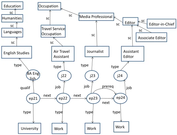
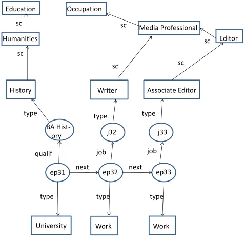
system allows users to create and maintain a chronological record of their learn-ing, work, and personal episodes — their “timelines” — with the aim of supporting learners in exploring learning and career opportunities and in planning and reflect-ing on their learnreflect-ing. Figures 8 and 9 illustrate a fragment of the data and metadata relating to two users’ timelines. The episodes within a timeline have a start and an end date associated with them (for simplicity these are not shown in the figure). Episodes are ordered by their start date — as indicated by edges labellednext. There are several types of episode, e.g.UniversityandWorkepisodes. Associ-ated with each type of episode are several properties — the figures show just two of these,qualif[ication]andjob6.

prereq

English Studies Air Travel

Assistant

Journalist Assistant

Editor

ep21 next ep22 next ep23 ep24

next

University Work Work Work

type type type type

j22

job

j23 j24

job job

BA Eng- lish

qualif

type _type type _type

Languages Travel Service _Occupation

Media Professional

Editor-in-Chief

Associate Editor Editor

Humanities

Education Occupation

sc

sc

sc sc

sc sc

sc

sc

sc sc

sc

Fig. 8 Fragment of data and metadata from Anne’s timeline

Suppose that Mary is studying for a BA in English and wishes to find out what possible future career choices there are for her. Timelines may have edges labelled prereqbetween episodes, indicating that the timeline’s owner believes that under-taking an earlier episode was necessary in order for them to be able to proceed to or achieve a later episode. So Mary might pose this CRPQ query,Q1:

(?E2,?P)<-(?E1,type,University),

(?E1,qualif.type,EnglishStudies), (?E1,prereq+,?E2),

(?E2,type,Work), (?E2,job.type,?P)

However, this will return no results even though Anne’s timeline in Figure 8 contains information that would be relevant to Mary. This is because, in practice, users may or may not createprereqmetadata relating to their timelines.

If Mary chooses to allow replacement of the edge labelprereqin her query by the labelnext(at an edit cost of 1, say), she can submit a variant ofQ1:

(?E2,?P)<-(?E1,type,University),

(?E1,qualif.type,EnglishStudies), APPROX (?E1,prereq+,?E2),

(?E2,type,Work), (?E2,job.type,?P)

The regular expressionprereq+can be approximated by the regular expression next.prereq*at edit distance 1 fromprereq+, returning the answer

(ep22,AirTravelAssistant)

Mary may judge this not to be relevant and may seek further results, at a further level of approximation. The regular expressionnext.prereq*can be approxi-mated bynext.next.prereq*, at edit distance 2 fromprereq+, returning the answers

(ep23,Journalist),(ep24,AssistantEditor)

Mary may judge these as being relevant, and she can then request the system to return the whole of Anne’s timeline for her to explore further.

The previous example took as input a starting timeline episode and explored possible future work choices. The next example additionally specifies an end goal and explores how someone might reach this from a given starting point.

Suppose now Mary knows she wants to become an Assistant Editor and would like to find out how she might achieve this, given that she’s done an English degree. Mary might pose this query,Q2:

(?E2,?P)<-(?E1,type,University),

(?E1,qualif.type,EnglishStudies),

APPROX(?E1,prereq+,?E2),(?E2,job.type,?P) APPROX(?E2,prereq+,?Goal),(?Goal,type,Work), (?Goal,job.type,AssistantEditor)

At edit distance 0 and 1 there are no results from Anne’s timeline. At edit distance 2, the answers

(ep22,AirTravelAssistant),(ep23,Journalist)

(?E2,?P)<-(?E1,type,University),

(?E1,qualif.type,EnglishStudies),

APPROX(?E1,prereq+,?E2),(?E2,job.type,?P) APPROX(?E2,prereq+,?Goal),(?Goal,type,Work), RELAX(?Goal,job.type,AssistantEditor)

which allows the system to relaxAssistant Editorto its parent classEditor, matching jobs such asAssistant Editor,Associate Editoretc., as well as in parallel approximating the two instances ofprereq+. Query results will be returned in increasing overall cost.

History Writer Associate Editor

ep31 next ep32 next ep33

University Work Work

type type type

j32 j33

job job

BA Hist- ory

qualif

type _type type

Media Professional

Editor Humanities

Education Occupation

sc sc

sc _sc

sc

sc

Fig. 9 Fragment of data and metadata from Bob’s timeline

As a further extension, suppose another user, Joe, wants to know what jobs simi-lar to being an Assistant Editor might be open to someone who has studied English or a similar subject at university. Joe may pose queryQ4which is the same asQ3 above but withRELAXin front of the second conjunct:

(?E2,?P)<-(?E1,type,University),

Suppose Joe sets the cost of relaxing a class to its parent class to 2 and replacing the labelprereqby the labelnextto 1. Then, the answers produced for query

Q4from the graphs in Figures 8 and 9 are shown in the table below. The first seven columns refer to the answers produced for each of the query conjuncts. For brevity, we do not show the full answer tuples, only the variable instantiations for each conjunct. We also show the relaxation distance (cost),rd, for the second and seventh conjucts, and the edit distance,ed, for the third and fifth conjuncts. In the table, “Air T.A.” stands for Air Travel Assistant, “Assist. Ed.” for Assistant Editor and “Assoc. Ed.” for Associate Editor. The final column shows the overall query answers and their overall distance (d) (which is the sum of therdandedvalues from the second, third, fifth and seventh conjuncts). For greater clarity, the tuples contributing to the first two answers areitalicisedand those contributing to the third answer are shown inbold.

?E1 ?E1,rd ?E1,?E2,ed ?E2,?P ?E2,?Goal,ed ?Goal ?Goal,rd ?E2,?P,d ep21 ep21,0 ep23,ep24,0 ep22,Air T.A. ep23,ep24,0 ep22 e24,0 ep23,Journalist,2

ep31 ep31,4ep21,ep22,1 ep23,Journalist ep21,ep22,1 ep23 e33,2 ep22,Air T.A.,6 ep22,ep23,1 ep24,Assist.Ed. ep22,ep23,1 ep24 e23,4 ep32,Writer,8 ep31,ep32,1 ep32,Writer ep31,ep32,1 ep32 e32,4

ep32,ep33,1 ep33,Assoc.Ed. ep32,ep33,1 ep33 e22,6

ep21,ep23,2 ep21,ep23,2

ep21,ep24,2 ep21,ep24,2

ep31,ep33,2 ep31,ep33,2

3.2 Automaton-Based Implementation Approach

We now discuss an automaton-based approach to evaluating regular path queries supporting both query approximation and query relaxation. The description is based on that from Poulovassilis and Wood (2010), with some modifications. We refer the reader to Poulovassilis and Wood (2010) and Poulovassilis et al (2016) for full details.

3.2.1 Computing approximate answers

Approximate matching of an RPQ queryQwith respect to a graphGis achieved by applying edit operations to sequences inL(R). Letqbe a sequence inL(R)andlbe a label inΣ∪Σ−∪ {type,type−}. We assume support for the following edit op-erations, each at some non-negative cost:insertionoflintoq,deletionoflfromq,

substitutionof some label other thanlbylinq. The cost of substitution is assumed to be less than the combined cost of insertion and deletion (otherwise the substi-tution operation would be redundant). Theinversionoperation is achieved through substitution, since this allows some labelainqto be substituted bya−. The

trans-positionoperation can be achieved by applying a substitution operation to each of

the two labels to be transposed.

Given an RPQQwith body(X,R,Y)and a graphG= (N,E), theapproximate

answerofQonGcan be computed as follows (the italicised terms are explained in

more detail below):

1. aweighted NFA,MR, recognisingL(R)is constructed fromR;

2. aquery automaton,MQ, is constructed fromQ;

3. anapproximate automaton,AQ, is constructed fromMQ;

4. theproduct automaton,H, ofAQandGis constructed;

5. one or more shortest path traversals are performed on H in order to find the approximate answer ofQonG.

Definition 1.Aweighted non-deterministic finite state automaton(weighted NFA)

MRrecognisingL(R)is the same as a normal NFA except that each transition and

each final state has a weight associated with it (all of which are initially zero). It can be constructed using Thompson’s construction (Aho et al (1974)), which makes use ofε-transitions.

Formally, MR= (S,Σ∪Σ−∪ {type,type−},δ,s0,Sf,ξ), where: S is the set of states; Σ∪ {type} is the alphabet of edge labels in G; δ ⊆S×Σ∪Σ−∪ {type,type−} ×N×Sis the transition relation;s0∈Sis the start state;Sfis the set

of final states, initially only consisting ofsf∈S; andξ is the final weight function mapping each state inSf to a non-negative number (initially, this will be zero for sf).

Thequery automaton MQforQisMRwith additional annotations on the initial

and final states: if X (resp.Y) is a constant c, then s0 (sf) is annotated with c;

Definition 2.Theapproximate automaton AQforQis constructed by first

construct-ing an automatonARfromMR. Formally,AR= (S,Σ∪Σ−∪ {type,type−},δ,s0,

Sf,ξ), withS,δ,s0andSf initially defined as in Definition 1.ARis then transformed

as follows:

• For each transition(s,a,0,t)∈δ (s6=t anda∈Σ∪Σ−∪ {type,type−}), the transition(s,ε,c_d,t)is added toδ, wherecdis the cost ofdeletion.

• Allε-transitions are removed fromδ using the method of Droste et al (2009). The method first computes theε-closure, which is the set of pairs of states con-nected by a sequence ofε-transitions along with the minimum summed weight for each such pair. Then for each pair(s,t)with weightwin theε-closure and each transition(t,b,0,u)∈δ (b=6 ε), a new transition(s,b,w,u)is added toδ. Ift∈Sf, thensis added toSf withξ[s] =wifξ[s]was previously undefined, or

withξ[s]set to the minimum ofξ[s]andwotherwise.

• For each transition(s,a,w,t)∈δ and labelb∈Σ∪Σ−∪ {type,type−}(b6=a), the transition(s,b,w+cs,t)is added toδ, wherecsis the cost ofsubstitution.

• For each state s∈S and label a∈Σ∪Σ−∪ {type,type−}, the transition (s,a,ci,s)is added toδ, whereciis the cost ofinsertion.

Theapproximate automaton AQforQis formed fromARby annotating the initial

and final states inAR with the annotations from the initial and final states,

respec-tively, inMQ.

Definition 3.Let AQ= (S,Σ∪Σ−∪ {type,type−},δ,s0,Sf,ξ) be an

approxi-mate automaton and G= (N,E) be a graph. G can be viewed as an automa-ton in which each node is both an initial and a final state. Theproduct automa-ton (Mendelzon and Wood (1989)), H, of AQ andG is the weighted automaton

(T,Σ∪Σ−∪ {type,type−},σ,I,F,ξ), whereI⊆T is a set of initial states and

F⊆T is a set of final states. The set of statesT is given by{(s,n)|s∈S∧n∈N}. The set of transitionsσconsists of transitions of the form

• ((s,n),a,c,(s0,n0))if(s,a,c,s0)∈δ and(n,a,n0)∈E, • ((s,n),a−,c,(s0,n0))if(s,a−,c,s0)∈δand(n0,a,n)∈E.

The set of initial statesIis given by{(s0,n)|n∈N}. The set of final statesF is given by{(sf,n)|(sf,n)∈T∧sf ∈Sf}.ξ is the final weight function mapping each states∈Fto a non-negative number. The annotations on initial and final states inHare carried over from the corresponding initial and final states inAQ.

Having formed the product automatonH, we can now compute the approximate answer ofQonG:

(i) Suppose first thatX is a constantv. Ifv∈/N, then the answer is empty. Ifv∈N, we perform a shortest path traversal ofH starting from the initial state(s0,v). Whenever we reach a final state(sf,n)inHwe outputn, providedn matchesthe

annotation on(sf,n)(recall that ifY is a constant the annotation onsf will be

that constant, and ifY is a variable the annotation will be the symbol∗). Noden

(ii)Now supposeXis a variable. In this case, we again perform a shortest path traver-sal ofH, outputting nodes as above, but this time starting from state(s0,v)for every nodev∈N.

Two optimisations to this naive traversal to avoid starting at every node of G

are described in Selmer et al (2015). Firstly, ifY is a constant, then(X,R,Y)is transformed to(Y,R−,X), whereR−is the reversal ofR, thus reverting to case (i) above. Otherwise (i.e. bothX andY are variables), we examine the labels on the transitions outgoing from the initial state ofAQ,s0, we retrieve fromGthe set of edges(v,l,w)matching these labels, and we perform the shortest path traversal starting from state(s0,v)for each such nodev.

The above evaluation can be accomplished “on-demand” by incrementally con-structing the edges of the product automatonHas required, rather than computing the entire graphH, as follows. Three collections are maintained (all initially empty):

• A setvisitedRcontaining tuples of the form(v,n,s), representing the fact that

nodenofGwas visited in statesofAQhaving started the traversal from nodev.

• A priority queuequeue_Rcontaining tuples of the form(v,n,s,d,f), ordered by non-decreasing values ofd, whered is the edit distance associated with visiting nodenin stateshaving started from nodev, and f is a flag denoting whether the tuple is ‘final’ or ‘non-final’.

• A listanswersRcontaining tuples of the form(v,n,d), whered is the smallest

edit distance of this answer tuple toQ, ordered by non-decreasing values ofd. This list is used to avoid returning an answer(v,n,d0)if there is already an answer (v,n,d)withd≤d0.

The evaluation of Q begins by adding to queue_R the initial tuple or tuples (v,v,s0,0,f)as detailed in (i) and (ii) above.

ProceduregetNextis then called to return the next query answer, in order of non-decreasing edit distance fromQ.getNextrepeatedly dequeues the first tuple ofqueue_R,(v,n,s,d,f), adding(v,n,s)tovisitedRif the tuple is not a final one,

untilqueue_Ris empty. If(v,n,s,d,f)is a final tuple and the answer(v,n,d0)has not been generated before for somed0, the triple(v,n,d)is returned after being added to answersR. If(v,n,s,d,f)is not final tuple, we enqueue(v,m,s0,d+d0,f))for each

transition d

0

→(s0,m)returned bySucc(s,n)such that(v,m,s0)6∈visitedR. Here,

theSuccfunction returns all transitions d

0

→(s0,m)such that there is an edge from (s,n)to(s0,m)inHwith costd0. WithinSucc, the functionnextStates(AQ,s,a)

returns the set of states inAQthat can be reached from stateson reading inputa,

ProceduregetNext(X,R,Y)

Input: query conjunct(X,R,Y)

Output: triple(v,n,d), wherevandnare instantiations ofXandY (1) whilenonempty(queueR)do

(2) (v,n,s,d,f)←dequeue(queueR)

(3) iff6=‘final’then

(4) add(v,n,s)tovisitedR

(5) foreach d

0

→(s0,m)∈Succ(s,n)s.t.(v,m,s0)6∈visitedRdo

(6) enqueue(queueR,(v,m,s0,d+d0,f))

(7) ifs is a final state and its annotation matches n and6 ∃d0.(v,n,d0)∈answersRthen

(8) enqueue(queueR,(v,n,s,d+ξ[s],‘final’))

(9) else

(10) if6 ∃d0.(v,n,d0)∈answersRthen

(11) append(v,n,d)toanswersR

(12) return(v,n,d)

(13) returnnull

FunctionSucc(s,n)

Input: statesofAQand nodenofG

Output: set of transitions which are successors of(s,n)inH (1) W←/0

(2) for(n,a,m)∈G and(p,d)∈nextStates(AQ,s,a)do

(3) add the transition→d (p,m)toW (4) returnW

3.2.2 Computing relaxed answers

We now describe how the relaxed answer of an RPQ queryQwith body(X,R,Y) can be computed, starting from the weighted NFAMRthat recognisesL(R). Below

we denote by ci the cost of applying rulei,i∈ {2,4,5,6}, from Figure 2 (since

queries and data graphs cannot contain edges labelledscandsp, rules 1 and 3 are inapplicable to them, although of course they are used in computing the closure of the RDF/S graph).

Given a weighted automatonMR= (S,Σ∪ {type},δ,s0,Sf,ξ)from which all

ε-transitions have been removed, and an ontologyKsuch thatK=extRed(K), an automaton MK

R = (S0,Σ∪ {type},τ,S0,S0f,ξ0)is constructed as described below.

The set of statesS0 includes the states inS as well as any new states defined be-low.S0andS0f are sets of initial and final states, respectively, withS0including the initial states0ofMR,S0f including the final statesSf ofMR, and both possibly

in-cluding additional states as defined below. We obtain therelaxed automatonofQ

final weight function mapping states inS0_f to a non-negative number. The transition relationτincludes the transitions inδ as well as any transitions added toτby the rules defined below. The rules below are repeatedly applied until no further changes toτandS0can be inferred. The process terminates because of the assumption that the subgraphs ofKinduced by edges labelledscandspare acyclic.

• (rule 2(i)) For each transition (s,a,d,t)∈τ and triple (a,sp,b)∈K, add the transition(s,b,d+c2,t)toτ.

• (rule 2(ii)) For each transition(s,a−,d,t)∈τ and triple(a,sp,b)∈K, add the transition(s,b−,d+c2,t)toτ.

• (rule 4(i)) For each transition(s,type,d,t)∈τsuch thatt∈S0_f,t is annotated withc, and(c,sc,c0)∈K, add toS0a new final statet0annotated withc0(unless there is already such a final state); add a copy of all oft’s outgoing transitions to

t0; and add the transition(s,type,d+c4,t0)toτ.

• (rule 4(ii)) For each transition transition(s,type−,d,t)∈τsuch thats∈S0,sis annotated withc, and(c,sc,c0)∈K, add toS0a new initial states0annotated with

c0(unless there is already such an initial state); add a copy of all ofs’s incoming transitions tos0; and add the transition(s0,type−,d+c4,t)toτ.

• (rule 5(i)) For each transition(s,a,d,t)∈τsuch thatt∈S0_f and(a,dom,c)∈K, add toS0a new final statet0annotated withc(unless there is already such a final state); add a copy of all oft’s outgoing transitions tot0; and add the transition (s,type,d+c5,t0)toτ.

• (rule 5(ii)) For each transition (s,a−,d,t)∈τ such thats∈S0 and(a,dom,c) ∈K, add toS0a new initial states0annotated withc(unless there is already such an initial state); add a copy of all ofs’s incoming transitions tos0; and add the transition(s0,type−,d+c5,t)toτ.

• (rule 6(i)) For each transition (s,a,d,t)∈τ such that s∈S0 and (a,range,c) ∈K, add toS0a new initial states0annotated withc(unless there is already such an initial state); add a copy of all ofs’s incoming transitions tos0; and add the transition(s0,type−,d+c6,t)toτ.

• (rule 6(ii)) For each transition(s,a−,d,t)∈τsuch thatt∈S0_f and(a,range,c) ∈K, add toS0a new final statet0annotated withc(unless there is already such a final state); add a copy of all oft’s outgoing transitions tot0; and add the transition (s,type,d+c6,t0)toτ.

Having constructed the relaxed automatonM_QK, its product automaton with the closure of the graphGis then constructed, and the computation proceeds similarly to cases (i) and (ii) for computing approximate answers above, except that in (i) if

3.3 System architecture and performance

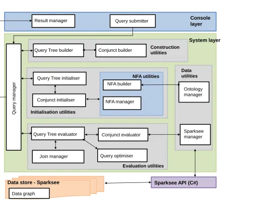
A prototype implementation of combined approximation and relaxation for CRPQs, calledOmega, is described in Selmer et al (2015) and Selmer (2016). Sparksee7_is used as the data store. The development was undertaken using the Microsoft .NET framework. The system comprises four components (see Figure 10): (i) theconsole

layer, to which queries are submitted and which displays the incrementally com-puted query results; (ii) thesystemlayer in which query plans are constructed, opti-mised and executed; (iii) the Sparksee API, which provides an interface for invoking data access methods to the data store; and (iv) the data store itself.

Query evaluation commences whenQuery submitter invokes Query manager, passing it a CRPQ query that is to be evaluated.Query managerinvokesQuery Tree

builderto construct the query tree, comprising inner nodes representing join

opera-tors and leaf nodes representing individual query conjuncts.Query Tree buildercalls

Conjunct builderto construct each leaf node of the query tree.Query managernext

passes the query tree toQuery Tree initialiser, which traverses the query tree in a top-down manner, begining at the root. WheneverQuery Tree initialiserencounters a leaf node in the query tree, it invokesConjunct initialiseron that conjunct. This in turn invokesNFA builderto construct the automaton corresponding to the conjunct’s regular expression. If the conjunct is approximated or relaxed, thenNFA manager

is invoked to produce an approximate or relaxed automaton, with the relevant edit or relaxation operators applied. For construction of a relaxed automaton,NFA man-agerinteracts withOntology manager, which stores the extended reduction of the ontology.Query managerthen invokesQuery Tree evaluator. This first invokes the

Query optimiserto transform the query tree into its final form for execution (see

below for a discussion of optimisation).Query Tree evaluatorthen traverses the op-timised query tree, starting from the leftmost leaf node, and proceeding upwards. If the current query tree node is a leaf, the ranked answers for the query conjunct are computed by invoking Conjunct evaluator. This module constructs the weighted product automaton,H, of the conjunct’s automaton with the (closure of) the data graphG. The construction ofH is incremental, withConjunct evaluatorinvoking

Sparksee managerto retrieve only those nodes and edges ofGthat are required in

order to compute the next batch ofkresults (for some predefined value ofk, default 100). If the current query tree node is a join,Query Tree evaluatorworks in con-junction withJoin managerto perform a ranked join of the answers returned thus far by its two children nodes. The join algorithm used is that described in Hurtado et al (2009b), itself adapted from Ilyas et al (2004). Once the root of the query tree has been reached, the processing terminates and the list of answers now holds the next

kresults, ranked by increasing distance.Query managerpasses this list toResult

managerwhich displays the results in ranked order.

Console layer

System layer

Data store - Sparksee

NFA builder Data utilities Evaluation utilities Qu e ry m a n a g e r Sparksee manager Query Tree builder

Query Tree initialiser NFA utilities Construction utilities

Data graph

Conjunct builder

Query Tree evaluator

Join manager Conjunct evaluator NFA manager Conjunct initialiser Query submitter Result manager Ontology manager

Sparksee API (C#)

Initialisation utilities

Query optimiser

Fig. 10 Omega System architecture

For constructing the automata, use is made of several data structures provided by the C5 Generic Collection library8, all of which have an amortized time complexity of O(1) for look-ups and updates:

• HashSet: a set of items (of some type T) implemented as a hash table with linear chaining.

• HashedLinkedList: A linked list of items (of some type T) with an addi-tional hash table to optimise item lookups within the list.

• HashDictionary: A hash table of typed (key,value) pairs.

The HashDictionary data structure is used to implement the automata, where the key is an integer representing a ‘from’ state s, and the value is a HashedLinkedListof tuples representing the transitions outgoing froms. The priority queuequeueRis also implemented by aHashDictionary. The key is

an integer-boolean variable (where the integer portion represents a distance and the boolean portion represents the final or non-final tuples at that distance). The value associated with each key, implemented using aHashedLinkedList, comprises tuples of the form(v,n,s,d,f), ordered by increasing values ofd, whered is the distance associated with visiting nodenin stateshaving started from nodev, and f

is a flag denoting whether the tuple is ‘final’ or ‘non-final’ Distinguishing between these two kinds of tuples in the priority queue allows the removal of ‘final’ tuples to be prioritised, so that answers may be returned earlier.

Readers are referred to Selmer et al (2015) and Selmer (2016) for further de-tails of the implementation and physical optimisations of theOmegasystem. Those works also report on a performance study of regular path queries with

tion and relaxation on several datasets sourced from the L4All system and from the SIMPLETAX and CORE portions of YAGO (Kasneci et al (2009)). The L4All data graphs used in the performance study were of size up to 220.8 MB for the closure of the data graph while the size of the closure of the YAGO data graph was 1.76 GB. Most of the APPROX and RELAX queries executed quickly on all datasets. How-ever, some of the APPROX queries on YAGO either failed to terminate or did not complete within a reasonable amount of time. This was mainly due to a large number of intermediate results being generated, due to theSuccfunction returning a large number of transitions which are then converted into tuples inGetNextand added to queueR. Some optimisations are explored in Selmer et al (2015) and Selmer (2016)

for such queries, enabling several — but not all — of the APPROX queries to ex-ecute faster. Future work includes making use of disk-resident data structures for queueRto guarantee the termination of APPROX queries with large intermediate

results, and using knowledge of the graph structure (e.g. to prioritise the evaluation of rarer paths within the graph) to reduce the amount of unnecessary processing. Another promising direction is to identify labels that are rare in the graph and to split the processing of a regular expression into smaller fragments whose first or last label is a rare label, as described in Koschmieder and Leser (2012) (but not for approximated/relaxed queries).

4

SPARQL

: Extending SPARQL with Approximation and

Relaxation

4.1 Example: Flexible Querying of RDF/S Knowledge Bases

Example 1.Suppose the user wishes to find the geographic coordinates of the

“Bat-tle of Waterloo” event by posing the following query on the YAGO knowledge base9, which is derived from multiple sources such as Wikipedia, WordNet and GeoNames:

PREFIX yago:<http://yago-knowledge.org/resource/>

PREFIX rdf:<http://www.w3.org/1999/02/22-rdf-syntax-ns#> SELECT * WHERE {

<http://yago-knowledge.org/resource/Battle_of_Waterloo> yago:happenedIn/(yago:hasLongitude|yago:hasLatitude) ?x }

This query uses theproperty pathsextension of SPARQL 1.1, including its con-catenation (/) and disjunction (|) operators. The above query does not return any answers since YAGO does not store the geographic coordinates of Waterloo.

The user may therefore choose to approximate the triple pattern in their query:

SELECT * WHERE {

APPROX(<http://yago-knowledge.org/resource/Battle_of_Waterloo> yago:happenedIn/(yago:hasLongitude|yago:hasLatitude)

?x ) }

YAGO does store directly the coordinates of the “Battle of Waterloo” event. So the system can apply an edit operation that deleteshappenedInfrom the property path, and the resulting query

SELECT * WHERE {

<http://yago-knowledge.org/resource/Battle_of_Waterloo> (yago:hasLongitude|yago:hasLatitude)

?x }

returns the desired answers, showing both high precision and high recall:

"4.4"ˆˆ<degrees>

"50.68333333333333"ˆˆ<degrees>

Example 2.Consider the following portionK= (NK,EK)of the YAGO ontology,

whereNKis

{hasFamilyName,hasGivenName,label,actedIn,Actor}

andEKis

{(hasFamilyName,sp,label),(hasGivenName,sp,label),

(actedIn,domain,actor)}

Suppose the user is looking for the family names of all actors who played in the film “Tea with Mussolini” and poses this query:

SELECT * WHERE {

?x yago:actedIn <http://yago-knowledge.org/resource/ Tea_with_Mussolini> .

?x yago:hasFamilyName ?z }

The above query returns only 4 answers, since some actors have only a single name (for example, Cher) while others have their full name recorded using thelabel property.

The user may choose to relax the second triple pattern in their query in an attempt to retrieve more answers:

SELECT * WHERE {

?x yago:actedIn <http://yago-knowledge.org/resource/ Tea_with_Mussolini> .

RELAX ( ?x yago:hasFamilyName ?z ) }

The system can now replace hasFamilyName by label, and the resulting query returns the given names of actors in that film recorded through the property hasGivenName(hence returning Cher), as well as actors’ full names recorded through the propertylabel: a total of 255 results.

Example 3.Suppose a user wishes to find events that took place in Berkshire in

1643 and poses the following query on YAGO (in the query, we use “Event” for simplicity but the actual URI is<wordnet_event_100029378>):

SELECT * WHERE {

?x rdf:type Event . ?x yago:on "1643-##-##" . ?x yago:in "Berkshire" }

This query returns no results because there are no property edges namedonorin in YAGO.

The user may choose to approximate the second and third triple patterns of their query:

SELECT * WHERE {

?x rdf:type Event .

APPROX ( ?x yago:on "1643-##-##" ) . APPROX ( ?x yago:in "Berkshire" ) }

The system can now substituteonbyhappenedOnDate(which does appear in YAGO) andinbyhappenedIn, giving the following query:

SELECT * WHERE {

?x rdf:type Event .

?x yago:happenedOnDate "1643-##-##" . ?x yago:happenedIn "Berkshire" }

This still returns no answers, sincehappenedIndoes not connect event instances directly to literals such as"Berkshire".

The user can choose to relax now the third triple pattern of the above query:

SELECT * WHERE {

?x rdf:type Event .

?x yago:happenedOnDate "1643-##-##" . RELAX ( ?x yago:happenedIn "Berkshire" )}

SELECT * WHERE {

?x rdf:type Event .

?x yago:happenedOnDate "1643-##-##" . ?x rdf:type Event }

Several answers are returned by this query, including the “Siege of Reading” that happened in 1643 in Berkshire, but also several events that did not happen in Berk-shire:

<http://yago-knowledge.org/resource/Battle_of_Olney_Bridge> <http://yago-knowledge.org/resource/Battle_of_Heptonstall> <http://yago-knowledge.org/resource/Siege_of_Reading> <http://yago-knowledge.org/resource/Torstenson_War> <http://yago-knowledge.org/resource/Battle_of_Alton>

<http://yago-knowledge.org/resource/Second_Battle_of_Middlewich> <http://yago-knowledge.org/resource/Kieft’s_War>

So the query exhibits better recall than the original query, but possibly low precision. The user can instead choose to approximate the third triple pattern:

SELECT * WHERE {

?x rdf:type Event .

?x yago:happenedOnDate "1643-##-##" . APPROX ( ?x yago:happenedIn "Berkshire" )}

The system can now insert the propertylabelthat connects URIs to their labels, giving the following query:

SELECT * WHERE {

?x rdf:type Event .

?x yago:happenedOnDate "1643-##-##" . ?x yago:happenedIn/label "Berkshire" }

This query now returns the only event recorded as occurring in 1643 in Berkshire i.e. the “Siege of Reading”. It exhibits both better recall than the original query and also high precision.

4.2 Query Rewriting-based Implementation Approach

For specifying the semantics of SPARQLARqueries we extend the notion of SPARQL query evaluation from returning a set of (exact) mappings to returning a set of map-ping/cost pairs of the form hµ,ci, where µ is a mapping and cis a non-negative number that indicates the cost of the answers arising from this mapping. Following on from the definitions of setsV,U andL, triples and triple patterns in Section 1, we have the following definitions (c.f. P´erez et al (2006)):

Definition 4 (Mapping).Amappingµ fromU LV toU Lis a partial function µ:

Definition 5 (Compatibility and Union of Mappings).Two mappingsµ1andµ2 arecompatibleif∀x∈var(µ1)∩var(µ2),µ1(x) =µ2(x). Theunionof two mappings µ=µ1∪µ2can be computed only ifµ1andµ2are compatible. The resultingµis a mapping such thatvar(µ) =var(µ1)∪var(µ2)and: for eachxinvar(µ1)∩var(µ2), µ(x) =µ1(x) =µ2(x); for eachxinvar(µ1)but not invar(µ2),µ(x) =µ1(x); and for eachxinvar(µ2)but not invar(µ1),µ(x) =µ2(x).

The unionof two sets of SPARQLAR _{query evaluation results,M}

1∪M2, com-prises the following set of mapping/cost pairs:

{hµ,ci | hµ,c1i ∈M1orhµ,c2i ∈M2, [email protected]µ,c2i ∈M2,c=c2if @c1.hµ,c1i ∈M1, andc=min(c1,c2)otherwise}.

In Cal`ı et al (2014) and Frosini et al (2015) aquery rewritingapproach is adopted for SPARQLARquery evaluation in which a SPARQLARqueryQis rewritten to a set of SPARQL 1.1 queries for evaluation. We summarise this approach here, refering the reader to those papers for further details.

To keep track of which triple patterns inQneed to be relaxed or approximated, such triple patterns are labelled withAfor approximation andRfor relaxation. The query rewriting algorithm starts by generating a queryQ0which returns the exact answer ofQ, i.e. ignoring any APPROX and RELAX operators. For each triple pat-ternhxi,Ri,yiiinQ0labelled withAorR, and each URIpthat appears inRi, a set of

new queries is constructed by applying all possible one-step edit operations or relax-ation operrelax-ations to p(these are the “first-generation” queries). To each such query

Q1is assigned the cost of applying the edit or relaxation operation that derived it. A new set of queries is constructed by applying a second step of approximation or re-laxation to each queryQ1(the “second-generation” queries), accumulating summa-tively the cost of the two edit or relaxation operations applied to obtain each query and assigning this cost to the query. The process continues for a bounded number of generations, accumulating summatively the cost of the sequence of edit or relaxation operations applied to obtain each query in theithgeneration. The rewriting process terminates once the cost of all the queries generated in a generation has exceeded a maximum valuem.

Algorithm 1:SPARQLAR_{Flexible Query Evaluation}

input : QueryQ; maximum costm; GraphG; OntologyK.

output: List of mapping/cost pairs,M, sorted by cost.

M:= /0;

foreachhQ0,costi ∈QRA(Q,m,K)do foreachµ∈SPARQLeval(Q0,G)do

M:=M∪ {hµ,costi}

returnM;

A formal study of the correctness and termination of the Query Rewriting Algo-rithm can be found in Frosini et al (2015) where the Rewriting AlgoAlgo-rithm itself is also specified in detail.

4.3 System architecture and performance

A prototype implementation of SPARQLAR_{is described in Frosini et al (2015). The}

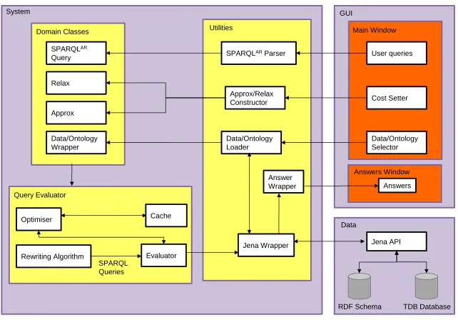
implementation is in Java and Jena is used for the SPARQL query execution. Figure 11 illustrates the system architecture, consisting of three layers: the GUI layer, the System layer, and the Data layer.

The GUI layer supports user interaction with the system, allowing queries to be submitted, costs of the edit and relaxation operators to be set, data sets and ontolo-gies to be selected, and query answers to be incrementally displayed to the user.

The System layer is responsible for the processing of the SPARQLAR queries. It comprises three components: the Utilities, containing classes providing the core logic of the system; the Domain Classes, providing classes relating to the construc-tion of SPARQLARqueries; and the Query Evaluator in which query rewriting, op-timisation and evaluation are undertaken.

The Data layer connects the system to the selected RDF dataset and ontology using the JENA API. Jena library methods are used to execute SPARQL queries over the RDF dataset and to load the ontology into memory. The RDF datasets are stored as a TDB database10 and the RDF schema can be stored in multiple RDF formats (e.g. Turtle, N-Triple, RDF/XML).

When a user query is submitted to the GUI, this invokes a method of the

SPARQLAR Parser to parse the query string and construct an object of the class

SPARQLARQuery. The GUI also invokes theData/Ontology Loaderwhich creates

an object of the classData/Ontology Wrapper, and theApprox/Relax Constructor

which creates objects of the classesApproxandRelax.

Once these objects have been initialised, they are passed to the Query Evaluator by invoking theRewriting Algorithm. This generates the set of SPARQL queries to be executed over the RDF dataset. The set of queries are passed to theEvaluator, which interacts with theOptimiserand theCacheto improve query performance.

Specifically, the answers of parts of queries are computed and stored in theCache, and these answers are retrieved from the Cache when theEvaluatorneeds these results. A SPARQLAR query is first split into two parts: the triple patterns which do not have APPROX or RELAX applied to them (the exact part) and those which have (the A/R part). The exact part is first evaluated and the results are cached. The query rewriting algorithm is then applied to the A/R part. Each triple pattern generated is evaluated individually, as also are all possible pairs of triple patterns, and the answers for each evaluation are cached. To avoid memory overflow, an upper limit is placed on the size of the cache. Finally, the overall results of a SPARQL query are obtained by joining subquery results already cached with those obtained by evaluating the rest of the query.

TheEvaluatoruses theJena Wrapperto invoke Jena library methods for

exe-cuting SPARQL queries over the RDF dataset. TheJena Wrapperalso gathers the query answers and passes them to the Answer Wrapper. Finally, the answers are displayed by theAnswers Window, in ranked order.

GUI System

Main Window

User queries

Cost Setter

Data/Ontology Selector Domain Classes

Jena Wrapper SPARQLAR Parser

Answer Wrapper Utilities

Query Evaluator

Approx/Relax Constructor

Data/Ontology Loader Relax

SPARQLAR

Query

Approx

Data/Ontology Wrapper

Rewriting Algorithm Evaluator Cache

SPARQL Queries Optimiser

Answers Answers Window

Jena API

RDF Schema TDB Database Data

Fig. 11 SPARQLAR_{system architecture}

A performance study using data generated from the Lehigh University Bench-mark (LUBM)11 is described in Cal`ı et al (2014). Three datasets were generated, the largest of which contained 673,416 triples (65MB). A larger-scale performance

study on the YAGO dataset is described in Frosini et al (2015). YAGO contains over 120 million triples which were downloaded and stored in a Jena TDB database. The size of the TDB database was 9.70 GB, and the nodes of the YAGO graph were stored in a 1.1 GB file.

The overall results show that the evaluation of SPARQLAR _{queries through a}

query rewriting approach is promising (see Cal`ı et al (2014), Frosini et al (2015) for details). The difference between the execution time of the exact form and the APPROXed/RELAXed forms of the queries is acceptable for queries with fewer than 5 conjuncts. For most of the other queries that were trialled, the simple caching technique described above also brings down the run times of their AP-PROXed/RELAXed forms to more reasonable levels. For more complex queries (e.g. involving combinations of Kleene closure and the wildcard symbol, “ ”, within a property path), more sophisticated optimisation techniques are needed.

Our ongoing work involves investigating optimisations to the query rewriting al-gorithm, since this can generate a large number of queries. In particular, we are studying the query containment problem for SPARQLARand how query costs im-pact on this. For example, for a queryQ=Q1ANDQ2it is possible to decrease the number of queries generated by the rewriting algorithm if we know thatQ1⊆Q2, in which case we can evaluateQ1rather thanQ. Other optimisations under inves-tigation include using statistics about path frequencies in the data graph to reorder the evaluation of triple patterns so as to evaluate first those returning fewer results; and using summaries of the data graph to avoid evaluating subqueries that we know, after evaluation on the graph summary, cannot return any answers. Also planned is a detailed comparison of this query rewriting approach to query approximation and relaxation with the “native” implementation of Omega described in the previous section.

5 Further Topics

5.1 User Interaction

In Section 3.1 we briefly discussed an application-specific prototype that provides a forms-based GUI for incrementally generating CRPQ queries, parts of which can optionally be approximated or relaxed, and for displaying ranked query results to the user. A detailed discussion of that prototype can be found in Poulovassilis et al (2012). An area of future work identified in that paper was how such systems might provide explanations to the user of how the overall ‘distance’ of each query result has been derived, based on the application of a sequence of edit and relaxation operations each of some cost specified by the user.