http://dx.doi.org/10.4236/am.2014.58115
Solution of Differential Equations with the
Aid of an Analytic Continuation of Laplace
Transform
Tohru Morita1, Ken-ichi Sato2
1Tohoku University, Sendai, Japan
2College of Engineering, Nihon University, Koriyama, Japan
Email: [email protected]
Received 4 February 2014; revised 4 March 2014; accepted 11 March 2014
Copyright © 2014 by authors and Scientific Research Publishing Inc.
This work is licensed under the Creative Commons Attribution International License (CC BY).
http://creativecommons.org/licenses/by/4.0/
Abstract
We discuss the solution of Laplace’s differential equation and a fractional differential equation of that type, by using analytic continuations of Riemann-Liouville fractional derivative and of Laplace transform. We show that the solutions, which are obtained by using operational calculus in the framework of distribution theory in our preceding papers, are obtained also by the present me-thod.
Keywords
Laplace’s Differential Equation, Kummer’s Differential Equation, Fractional Differential Equation, Laplace Transform, Analytic Continuation via Hankel’s Contour
1. Introduction
Yosida [1] [2] discussed the solution of Laplace’s differential equation, which is a linear differential equation, with coefficients which are linear functions of the variable. In recent papers [3] [4], we discussed the solution of that equation, and fractional differential equation of that type. The differential equations are expressed as
(
)
2( ) (
)
( ) (
) ( )
( )
2 2 0 R 1 1 0 R 0 0 , 0,
a t+b ⋅ D u tσ + a t+b ⋅ D u tσ + a t+b u t = f t t> (1.1) for σ=1 and σ =1 2. Here a bl, l for l=0,1, 2 are constants, and 0
( )
l R
D u tσ are the Riemann-Liouville fractional derivatives to be defined in Section 2.
[ ]b c, :=
{
n∈ b≤ ≤n c}
for a∈ and b c, ∈ satisfying b<c. If n∈>0, 0
( )
( )
d d
n n
R n
D u t u t
t
= , and
( ) ( )
0
0D u tR =u t . We use x for x∈, to denote the least integer that is not less than x. In the present paper,
the variable t is always assumed to take values on >0.
Yosida [1] [2] studied the Equation (1.1) for σ=1 with f t
( )
=0, by using Mikusiński’s operational cal-culus [5]. In [3] [4], operational calculus in terms of distribution theory is used, which was developed for the ini-tial-value problem of fractional differential equation with constant coefficients in our preceding papers [6] [7]. In [3], the derivative is the ordinary Riemann-Liouville fractional derivative, so that the fractional derivative of a function u t( )
exists only when u t( )
is locally integrable on >0, and the integral( )
1 0u t dt
∫
converges. Practically, we adopt Condition B in [3], which isCondition 1. u t
( )
and f t( )
in (1) are expressed as a linear combination of gν( )
t for ν∈>0.Here gν
( )
t is defined by( )
( )
1 1, 0,
gν t tν t
ν
−
= >
Γ (1.2)
for ν∈ <1, where Γ
( )
ν is the gamma function.We then express u t
( )
as follows:( )
( )
1
1 ,
S
u t uν gν t
ν∈ −
=
∑
(1.3)where uν −1∈ are constants, and S1 is a set of ν∈>0.
In a recent review [8], we discussed the analytic continuations of fractional derivative, where an analytic continuation of Riemann-Liouville fractional derivative of function u t
( )
is such that the fractional derivative exists when u t( )
is locally integrable on >0, even when the integral( )
1 0u t dt
∫
diverges.In [4], we adopted this analytic continuation of Riemann-Liouville fractional derivative, and the following condition, in place of Condition 1.
Condition 2. u t
( )
and f t( )
in (1.1) are expressed as a linear combination of gν( )
t for ν∈S, where S is a set of ν∈>−M<1 for some M∈>−1.We then express u t
( )
as follows;( )
1( )
.S
u t uν gν t
ν∈ −
=
∑
(1.4)In [3] [4], we take up Kummer’s differential equation as an example, which is
( ) (
)
( )
( )
2 2
d d
0, 0,
d d
t u t c t u t a u t t
t t
⋅ + − ⋅ − ⋅ = > (1.5)
where a c, ∈ are constants. If c∉, one of the solutions given in [9] [10] is
(
)
( )
( )
1 1
0
; ; : ,
!
n n
n n
a
F a c t t
c n
∞ =
=
∑
(1.6)where
( )
a n=∏
kn−=10(
a+k)
for a∈ and n∈>0, and( )
a 0=1. The other solution is(
)
1
1 1 1; 2 ; .
c
t− ⋅ F a c− + −c t (1.7) In [3], if c<2, we obtain both of the solutions. But when c≥2, (1.7) does not satisfy Condition 1 and we could not get it in [3]. In [4], we always obtain both of the solutions. In [1] [2], Yosida obtained only the solu- tion (1.7).
We now study the solution of a differential equation with the aid of Laplace transform. Then it is required that there exists the Laplace transform of the function u t
( )
to be determined.When we consider the Laplace transform of a function f t
( )
which is locally integrable on >0, weas-sume the following condition.
Condition 3. There exists some λ∈>0 such that
( )
e 0 tf t −λ → as t→ ∞.
Let f t
( )
be locally integrable on >0 and satisfy Condition 3, and the integral( )
1 0f t dt
then denote its Laplace transform by f s
( )
= f t( )
, so that( )
( )
: 0( )
estd . f s = f t =∫
∞f t − t (1.8)
The Laplace transform, gν
( )
s , of gν( )
t for ν∈>0 is then given by( )
.gν s =s−ν (1.9) Let u t
( )
expressed by (1.3) satisfy Condition 3, and let its Laplace transform u s( )
be given by( )
1
1 .
S
u s uν sν
ν
− − ∈
=
∑
(1.10)
Then we can show that we are able to solve the problems solved in [3], with the aid of Laplace transform. When u t
( )
satisfies Conditions 2 and 3, Laplace transform is not applicable.In [4], we adopted an analytic continuation of Riemann-Liouville fractional derivative, by which we could solve the differential equation assuming Condition 2. The analytic continuation is achieved with the aid of Pochhammer’s contour, which is used in the analytic continuation of the beta function.
We now introduce the analytic continuation of Laplace transform with the aid of Hankel’s contour, which is used in the analytic continuation of the gamma function. We then show that (1.9) is valid for ν∈ <1, and
that if u t
( )
expressed by (1.4) satisfies Condition 3, and its analytic continuation of Laplace transform of( )
u t , which we denote by u sˆ
( )
, is given by( )
1ˆ ,
S u s uν sν
ν
− − ∈
=
∑
(1.11)then we can solve the problems solved in [4], with the aid of the analytic continuation of Laplace transform. In Section 2, we prepare the definition of analytic continuations of Riemann-Liouville fractional derivative and of Laplace transform, and then explain how the equation for the function u t
( )
and its fractional derivative in (1.1) are converted into the corresponding equation for the analytic continuation of Laplace transform, u sˆ( )
, of u t( )
, and also how u sˆ( )
is converted back into u t( )
. After these preparations, a recipe is given to be used in solving the fractional differential Equation (1.1) with the aid of the analytic continuation of Laplace transform in Section 3. In this recipe, the solution is obtained only when a2 ≠0 and b2 =0. When1 2
σ= , b1=0 is
also required. An explanation of this fact is given in Appendices C and D of [3]. In Section 4, we apply the rec-ipe to (1.1) where σ =1 and a0 =0, of which special one is Kummer’s differential equation. In Section 5, we
apply the recipe to the fractional differential equation with 1 2
σ= , assuming a0=0.
In Section 6, comments are given on the relation of the present method with the preceding one developed in [4], and on the application of the analytic continuation of Laplace transform to the differential equations with constant coefficients.
2. Formulas
Lemma 1. Let gν
( )
t be defined by (1.2). Then for ν∈<1,( )
1( )
, 0.t g⋅ ν t = ⋅ν gν+ t t> (2.1) Proof. By (1.2), for ν∉<1,
( )
( )
(
)
1( )
1
1
t g⋅ ν t =Γν tν =Γ +νν tν = ⋅ν gν+ t .
2.1. Analytic Continuation of Riemann-Liouville Fractional Derivative Let a function f t
( )
be locally integrable on >b for b∈, and let( )
1
d b
b f t t
+
∫
exist. We then define the Riemann-Liouville fractional integral, bDR f t( )
λ −
, of order
0 λ∈> by
( )
( ) (
1)
1( )
d , .
t
bDR f t b t x f x x t b
λ λ
λ
−
− = − >
Γ
∫
We then define the Riemann-Liouville fractional derivative, bD f tR
( )
β
, of order β∈, by
( )
d( )
, ,
d N
N
bD f tR tN bDR f t t b
β = β− >
(2.3) if it exists, where N=max
{
β , 0}
, and bD f tR0( )
= f t( )
for t>b.For ν,t>0 and b=0, we have
( )
( )
10
1
, ,
0, .
R
g t
D gβ ν t ν β ν β
ν β
− < <
− ∈
=
− ∈
(2.4)
If we assume that β = −λ takes a complex value, 0D gR
( )
tβ ν
by definition (2.2) is analytic function of β in the domain Reβ<0, and 0D gR
( )
tβ
ν defined by (2.3) is its analytic continuation to the whole complex
plane. If we assume that ν also takes a complex value, 0D gR
( )
tβ
ν defined by (2.3) is an analytic function of
ν in the domain Reν>0. The analytic continuation as a function of ν was also studied. The argument is concluded that (2.4) should apply for the analytic continuation via Pochhammer’s contour, even in Reν≤0 except at the points where ν∈<1; see [8].
We now adopt this analytic continuation of 0D gR
( )
tβ
ν to represent 0D gR
( )
tβ
ν , and hence we accept the
following lemma.
Lemma 2. Formula (2.4) holds for every β∈, ν∈ <1.
By (1.4) and (2.4), we have
( )
( )
1
0 1
,
. R
S
D u tβ uν gν β t
ν ν β <
− − ∈ − ∉
=
∑
(2.5)
For u t
( )
defined by (1.4), we note that 0( )
M RD− u t is locally integrable on >0.
2.2. Analytic Continuation of Laplace Transform
The gamma function Γ
( )
z for z∈ satisfying Rez>0, is defined by Euler’s second integral:( )
10 e d .
z t z ∞t − − t
Γ =
∫
(2.6) The analytic continuation of Γ( )
z for z∈ is given by Hankel’s formula:( )
e π 1 1e d ,2 sinπ H
i z z
C z
i z
ζ
ζ ζ
− − −
Γ =
∫
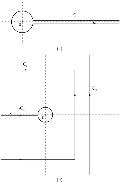
(2.7)where CH is Hankel’s contour shown inFigure 1(a).
We now define an integral transform f sˆ
( )
=Hf t( )
of a function f t( )
which satisfies the followingcondition.
Condition 4. f z
( )
is expressed as f z( )
z 1f z1( )
γ −
= on a neighborhood of >0, for 0≤argz<2π,
where γ∈ <1, and f1
( )
z is analytic on the neighborhood of >0.Let f t
( )
satisfy Conditions 3 and 4. Then we define f sˆ( )
for γ∈ <1, by f sˆ( )
=Hf t( )
, where( )
e π 1( )
e d , 2 sinπ Hi s
H f t C f
i
γ ζ ζ ζ
γ
− −
=
∫
(2.8)
for γ ∈ , and
( )
1( )
1
lim i ,
i
H H
n
f t tγ f t
γ
−
→
= ⋅
(2.9)
for γ = ∈n >0,γi∈ .
Lemma 3. Let f t
( )
satisfy Condition 4. Then f s defined by ˆ( )
(2.8) is an analytic continuation of f s( )
, which is defined by (1.8) for Reγ >0, as a function of γ .Proof. The equality f sˆ
( )
= f s( )
when Reγ >0 is proved in the same way as the equality of Γ( )
z given by (2.6) and by (2.7) for Rez>0; see e.g. ([11], Section 12.22). The analyticity of f sˆ( )
and of f s( )
is proved as in ([11], Sections 5.31, 5.32). (a)
[image:5.595.213.415.85.390.2](b)
Figure 1. (a) Hankel’s contour CH, and (b) contours CI, −CH and CB which appear in (2.12), (2.15) and
(2.16).
( )
ˆ ,
gν s =s−ν (2.10)
( )
d( )
ˆ ,
d
H t g t g s
s
ν ν
⋅ = −
(2.11)
( )
1 1e d e d ,
2π H 2π I
st st
C C
g t s s s s
i i
ν ν
ν =
∫
− − =∫
− (2.12)where −CH and CI are two of the contours shown inFigure 1(b).
Proof. Formula (2.8) for f t
( )
=gγ( )
t gives( )
π 1( )
1 1ˆ e e d ,
2 sinπ H
i s
C
g s s
i
γ γ ζ γ
ν = − γ
∫
Γ γ ζ − − ζ = − (2.13)for γ ∈ . The last equality in (2.13) is due to (1.9). By using (2.1) and (2.10), the lefthand side of (2.11) is
expressed as
( )
1( )
1
d d
ˆ
d d
H g t s s g s
s s
ν ν
ν ν
ν ν − − −
+
⋅ = ⋅ = − = −
. By replacing s, γ and ζ in (2.13), by t, 1
ν
− + and e iπ
s
−
, respectively, we obtain the first equality of (2.12) for ν∉, with the aid of the formula
( ) (
)
π 1
sinπz= Γ z Γ −z . The equality for ν∈>0 is obtained by continuity.
Theorem 1. Let f t
( )
satisfy Conditions 3 and 4 for γ >0, and u t( )
be expressed as( )
( )
( )
0
1 ,
S
u t uν gν t f t
ν∈ −
=
∑
+ (2.14)( )
1 ˆ( )
1 ˆ( )
: e d ,
2π I
st
H C
u t u s u s s
i
−
= =
∫
(2.15)where CI is a contour shown inFigure 1(b). Here it is assumed that f sˆ
( )
is analytic to the right of the verticalline on CI, and is so above and below the upper and lower horizontal lines, respectively, on CI.
Proof. For f t
( )
, the usual Laplace inversion formula applies, so that( )
1 ˆ( )
1 ˆ( )
e d e d ,
2π B 2π I
st st
C C
f t f s s f s s
i i
=
∫
=∫
(2.16)where CB is a contour shown inFigure 1(b). Here it is assumed that f sˆ
( )
is analytic to the right of the contourCB. By using this with (2.10) and (2.12), we confirm (2.15).
Lemma 5. Let f t
( )
satisfy Conditions 3 and 4 with an entire function f t1( )
. Then( )
( )( ) (
)
10
ˆ 0 .
!
n n
n
n
f s s f s
n
γ ∞ γ
− −
=
Γ +
=
∑
(2.17)Lemma 6. Let u sˆ
( )
be expressed in the form of (1.11). Then the Laplace inversion u t( )
is given by (1.4), provided that the obtained u t( )
satisfies the conditions for f t( )
in Lemma 5, or it is a linear combination of such functions.Lemma 7. Let u t
( )
satisfy the conditions for f t( )
in Lemma 5. Then( )
( )
( )
1 1
1
0 1 1
, , 1 , ˆ ˆ , H R S S k k
k k S
D u t u g s u s
s u s u s
β ν β
ν ν β ν ν ν β ν ν β
β β β < < >− − + − − − ∈ − ∉ ∈ − ∉ − − ∈ − ∈ = = = −
∑
∑
∑
(2.18)( )
( )
0 0 d . dH t D u tR H D u tR
s
β β
⋅ = −
(2.19)
Proof. By using (2.5) and Lemma 4, we obtain these results.
3. Recipe of Solving Laplace’s Differential Equation and Fractional Differential
Equation of That Type
We now express the differential Equation (1.1) to be solved, as follows:
(
)
0( )
( )
0
, 0,
m
l
l l R
l
a t b D u tσ f t t
=
+ ⋅ = >
∑
(3.1)where 1 2
σ = or σ=1, and m=2. In Sections 4 and 5, we study this differential equation for σ =1 and
this fractional differential equation for 1 2
σ = , respectively.
We now apply the integral transform H to (3.1). By using (2.18) and (2.19), we then obtain
( )
d( )
( ) ( )
ˆ( ) ( )
ˆ ˆ ˆ ,
d
A s u s B s u s f s v s
s
− + = + (3.2)
where
( )
( )
(
)
0 1 0 , , m l l l m l l l l lA s a s
B s l a s b s
σ σ σ σ = − = = ⋅ = − ⋅ ⋅ + ⋅
∑
∑
(3.3)( )
* * 1 1 1 =1 ˆ . m k kl l k l l k
l k k
v s a k uσ− − s − b uσ− − s
Here *:=
{
k∈>−1 lσ− ∉k <1}
.Lemma 8. The complementary solution (C-solution) of Equation (3.2) is given by u sˆ
( )
=C1⋅φˆ( )
s , where C1is an arbitrary constant and
( )
2( )
( )
ˆ s C exp sB d , A
ξ
φ ξ
ξ
= ⋅
∫
(3.5)where the integral is the indefinite integral and C2 is any constant.
Lemma 9. Let φˆ
( )
s be the C-solution of (3.2), and uˆν*( )
s be the particular solution (P-solution) of (3.2), when the inhomogeneous term is s−ν for ν∈. Then( )
( )
( ) ( )
( )
*
3
ˆ ˆ
ˆ d ,
ˆ
s
u s s C s
A
ν
ν φ ξ ξ φ
ξ φ ξ
−
= −
∫
+ ⋅ (3.6)where C3 is any constant.
Since f t
( )
in (3.1) satisfies Condition 2 and v sˆ( )
is given by (3.4), the P-solution u sˆ( )
of (3.2) is ex-pressed as a linear combination of uˆν*( )
s for ν∈>−M for M∈>−1, and of( )
*
ˆ k
u− s for k∈>−1,
respec-tively.
The solution u sˆ
( )
of (3.2) is converted to a solution u t( )
of (3.1) for t>0, with the aid of Lemma 6.4. Laplace’s and Kummer’s Differential Equations
We now consider the case of σ=1, m=2, a2≠0, a1≠0, and a0=b2=0. Then (3.1) reduces to
( ) (
)
( )
( )
( )
2
2 2 1 1 0
d d
, 0.
d d
a t u t a t b u t b u t f t t
t t
⋅ + + ⋅ + ⋅ = > (4.1)
By (3.3) and (3.4), A s
( )
, B s( )
and v sˆ( )
are( )
(
)
( ) (
)
2 1
2 1 2
2
1 2 0 1
, ,
2 ,
a A s a s a s a s s
a
B s b a s b a
α α
= + = + =
= − + −
(4.2)
( ) (
2 1)
0ˆ .
v s = − +a b u (4.3) 4.1. Complementary Solution of (3.2) and (4.1)
In order to obtain the C-solution φˆ
( )
s of (3.2) by using (3.5), we express B s( ) ( )
A s as follows:( )
( )
1 2 , B sA s s s
γ γ
α
= +
+ (4.4) where
0 0
1 1
1 2 1 2
2 1 2 1
2, b 1, b 1.
b b
a a a a
γ +γ = − γ = − γ = − − (4.5)
By using (3.5), we obtain
( )
1(
)
2 1 2(
1)
2 1 2 20
ˆ 1 n n,
n
s s s s s s s
n
γ γ
γ γ γ γ γ γ
φ α + α − + ∞ α −
=
= + = + =
∑
(4.6)in the form of (2.17) or (1.11), where
( ) ( )
1 ! nn
n n
γ
γ − −
=
for γ∈ and n∈>−1 are the binomial
coeffi-cients.
( )
( )
1 2 1 2(
)
1 1
0 1 2
1
n n
n
u t C t C t t
n n
γ γ γ
φ α γ γ ∞ − − − = = ⋅ = ⋅
Γ − −
∑
(4.7)(
)
1 2 1(
)
1 1 1 2 1 2
1 2
1
; ; .
C t γ γ F γ γ γ αt
γ γ
− − −
= ⋅ ⋅ − − − −
Γ − − (4.8)
Remark 1. In Introduction, Kummer’s differential equation is given by (1.5). It is equal to (4.1) for a2 =1,
1 1
a = − , b1=c and b0 = −a. In this case,
2 c a 1, 1 a 1, 1 2 c 2, 1.
γ = − − γ = − γ +γ = − α = − (4.9)
We then confirm that the expression (4.8) for c∉>1 agrees with (1.7), which is one of the C-solutions of
Kummer’s differential equation given in [9] [10]. 4.2. Particular Solution of (3.2)
We now obtain the P-solution of (3.2), when the inhomogeneous term is equal to s−ν for ν∈.
When the C-solution of (3.2) is φˆ
( )
s , the P-solution of (3.2) is given by (3.6). By using (4.2) and (4.6), the following result is obtained in [3]:( )
(
)
(
)
( )
2 1 2 1 2 1 * 3 1 1 2 1 * , 1 0 2 ˆ ˆ d 1 , s n n n nu s s s C s
a
s C s
a
ν γ
γ
ν γ γ
ν
γ γ ν
ξ
α ξ φ
ξ ξ α
α − + + ∞ − − − + + = = − + + ⋅ + = ⋅
∫
∑
(4.10) where 1 2 1 1 * ,0 1 2
1 1
.
n n p p
k
p p
C
k n k n k p p
= − − = − − + +
∑
(4.11)Lemma 10. When p1+p2∉<1, 1 2
* ,
nCp p defined by (4.11) is expressed as
( )
1 2 * , 1 2 1nnCp p
p p
− =
+ 1 2
† , , nCp p
⋅ (4.12)
where
( )
(
)
1 2 2 † , 1 2 . 1 n n p pn
p C
p p
=
+ + (4.13)
This lemma is proved in [3]. In fact, (4.11) is the partial fraction expansion of
1 2
* ,
nCp p given by (4.12) as a
function of p2.
Applying Lemma 6 to (4.10), and using (4.12), we obtain
Theorem 2.Let ν∈ <0, 1+ + + ∉ν γ γ1 2 <1, and let f t
( )
=gν( )
t for t>0. Then we have a P-solu-tion u tν*
( )
of (4.1), given by( )
(
)
*
2 1 2
1 1 u t
a
ν = ⋅ + + +ν γ γ uν†
( )
t , (4.14)where
( )
(
(
)
1)
(
) (
)
†
0 1 2
1
2 1
n n
n n
u t t t
n
ν ν
ν γ
α
ν γ γ ν
∞ =
+ +
= −
+ + + ⋅Γ + +
∑
(4.15)(
)
2 2(
1 1 2)
1
1 ,1; 2 , 1; .
1 t F t
ν ν γ ν γ γ ν α
ν
= ⋅ + + + + + + −
Γ + (4.16)
Here
(
)
( ) ( )
( ) ( )
1 22 2 1 2 1 2 0
1 2 , ; , ; ! n n n n n n a a
F a a b b x x
b b n
∞ =
4.3. Complementary Solution of (4.1)
By (4.3) and (4.5), v sˆ
( )
=a2⋅ + +(
1 γ1 γ2)
⋅u0. When f sˆ( )
=0 and v sˆ( )
≠0, the P-solution of (3.2) is givenby
( )
(
)
*( )
2 1 2 0 0
ˆ 1 ˆ .
u s =a ⋅ + +γ γ ⋅ ⋅u u s (4.17)
By using (4.14) for ν =0, if 1+ +γ γ1 2∉<1, we obtain a C-solution of (4.1):
( )
†( )
(
)
0 0 0 1 1 1 1; 2 1 2; .
u t =u u⋅ t =u ⋅ F +γ + +γ γ −αt (4.18) In Section 4.1, we have (4.7), that is another C-solution of (4.1). If we compare (4.7) with (4.15), when
1 2 1
γ +γ ∉>− , it can be expressed as
( )
†1 2( )
1 1 1 .
C ⋅φ t =C u⋅ − − −γ γ t (4.19) Proposition 1. When γ1+γ2∉, the complementary solution of (4.1) is given by the sum of the righthand
sides of (4.8) and of (4.18), which are equal to
( )
1 2
†
1 1
C u⋅ − − −γ γ t and u u0⋅ †0
( )
t , respectively.Remark 2. As stated in Remark 1, for Kummer’s differential equation, γ1 and γ2 are given in (4.9), and
1 1 2
1+γ =a, 2+ +γ γ =c, α = −1. (4.20) We then confirm that if c∉, the set of (4.8) and (4.18) agrees with the set of (1.6) and (1.7).
5. Solution of Fractional Differential Equation (3.1) for
σ
= 1 2
In this section, we consider the case of 1 2
σ = , m=2, a2 ≠0, a1 ≠0, a0 =b2 = =b1 0 and b0 ≠0. Then
the Equation (3.1) to be solved is
( )
1 2( )
( )
( )
2 0 R 1 0 R 0 , 0.
a t⋅ D u t +a t⋅ D u t + ⋅b u t = f t t> (5.1) Now (3.3) and (3.4) are expressed as
( )
(
)
( )
1 2 1 2 1 2 1 2 1 2
2 1 2
0 2 1
, ,
1 , 2
a
A s a s a s a s s
a
B s b a a s
α α
−
= + = + =
= − −
(5.2)
( )
1(
)
1 2 2 0ˆ 1 .
M
k k k
v s a k u − − s
=
= −
∑
+ ⋅ (5.3)5.1. Complementary Solution of (3.2) By using (5.2), B s
( ) ( )
A s is expressed as( )
( )
1 2 1 21 1 22 ,B s s
A s s s
γ γ
α
−
= +
+
(5.4) where
0 0
1 2 1 2
2 2
1 1
1, , .
2 2
b b
a a
γ +γ = − γ = − γ = − (5.5)
By (3.5), the C-solution φˆ
( )
s of (3.2) is given by( )
1(
1 2)
22 1 2(
1 2)
22 1 2 2 2 02
ˆ 1 n n .
n
s s s s s s s
n
γ γ
γ γ γ γ γ γ
φ α + α − + ∞ α −
=
= + = + =
∑
(5.6)( )
( )
1 2 1 2 21 1
0
1 2
2 1
. 2
n n n
u t C t C t t
n n
γ γ γ
φ α
γ γ
∞ − − −
=
= ⋅ = ⋅
Γ − −
∑
(5.7)5.2. Particular Solution of (3.2) and (5.1)
By using the expressions of A s
( )
and φˆ( )
s given by (5.2) and (5.6) in (3.6), we obtain the P-solution of (3.2), when the inhomogeneous term is x−ν for ν∈ satisfying 2(
ν γ+ +1 γ2)
∉<1:( )
(
)
(
)
( )
2 1
2 1
2 1
2
* 1 2
3 1 2
1 2 1 2
2
* 2
2 ,2 2 0
2
ˆ
ˆ d
2
,
s
n n
n n
u s s s C s
a
s C s
a
ν γ
γ
ν γ γ
ν
γ γ ν
ξ
α ξ φ
ξ ξ α
α
− + +
∞
− −
+ =
= − + + ⋅
+
= ⋅
∫
∑
(5.8)
where
2 1
* 2 ,2 2
nCγ γ+ν is defined by (4.11) and is given by (4.12).
By applying Lemma 6 to this, we obtain the following theorem.
Theorem 3. Let ν∈, 2ν∉<1, 2
(
ν γ+ +1 γ2)
∉<1, and let f t( )
=gν( )
t . Then we have a P-solution( )
*
u tν of (5.1), given by
( )
(
)
*
2 1 2
1 u t
a
ν = ⋅ + +ν γ γ uν†
( )
t , (5.9)where
( )
(
(
1)
)
( )
† 1 2
0 1 2
2 2 1
.
1 2 2 2
2
n n n
n n
u t t t
n
ν ν
ν γ
α
ν γ γ ν
∞ −
=
+
= ⋅ −
+ + + Γ +
∑
(5.10)5.3. Complementary Solution of (5.1)
We obtain the solution u tν*
( )
only for 2ν∉<1. When v sˆ( )
is given by (5.3) with nonzero values of u1 2− −k 2,Theorem 2 does not give a solution of (5.1). Hence u t
( )
given by (5.7) is the only C-solution of (5.1). If we compare (5.7) with (5.10), we obtain the following proposition.Proposition 2. Let 2
(
γ1+γ2)
∉>−1. Then the C-solution of (5.1) is given by( )
†1 2( )
1 1 .
C ⋅φ t =C u⋅ − −γ γ t (5.11)
6. Concluding Remarks
6.1. Solution with the Aid of Distribution Theory
In [4], the solution of (3.1) is assumed to be expressed as (1.4). In distribution theory, the differential equation for the distribution u t
( )
=u t H t( ) ( )
is set up, where H t( )
=1 for t>0 and H t( )
=0 for t≤0. Then it is expressed as u t( ) ( ) ( )
u Dˆ t Su 1D( )
tν ν ν
δ −δ
− ∈
= =
∑
, where D−ν is the derivative of order −ν in the space of
R′
of distributions. In [4], after obtaining u Dˆ
( )
, u t( )
is obtained by using Neumann series expansion. In the present paper, u sˆ( )
is the analytic continuation of Laplace transform of u t( )
. After obtaining u sˆ( )
, we obtain u t( )
for t>0 by Laplace inversion.The steps of solution in [4] and the present paper are closely related with each other, and one may use a favo-rite one. One difference is that Condition 3 is assumed in the present paper but is not required in [4].
6.2. Solutions of Differential Equations with Constant Coefficients
We now consider the differential equation given by (3.1), where a2=a1=a0=0. Then assuming that the
continu-ation of Laplace transform of u t
( )
, u sˆ( )
. If it can be expressed as (1.11), then u t( )
is given by its Laplace inverse (1.4). If we take account of Section 6.1, we confirm that the results obtained in [7] are obtained by Lap-lace inversion.References
[1] Yosida, K. (1983) The Algebraic Derivative and Laplace’s Differential Equation. Proceedings of Japan Academy, 59, 1-4. http://dx.doi.org/10.3792/pjaa.59.1
[2] Yosida, K. (1982) Operational Calculus. Springer-Verlag, New York, Chapter VII.
[3] Morita, T. and Sato, K. (2013) Remarks on the Solution of Laplace’s Differential Equation and Fractional Differential Equation of That Type. Applied Mathematics, 4, 13-21. http://dx.doi.org/10.4236/am.2013.411A1003
[4] Morita, T. and Sato, K. (2013) Solution of Laplace’s Differential Equation and Fractional Differential Equation of That Type. Applied Mathematics, 4, 26-36. http://dx.doi.org/10.4236/am.2013.411A1005
[5] Mikusiński, J. (1959) Operational Calculus. Pergamon Press, London.
[6] Morita, T. and Sato, K. (2006) Solution of Fractional Differential Equation in Terms of Distribution Theory. Interdis-ciplinary Information Sciences, 12, 71-83.
[7] Morita, T. and Sato, K. (2010) Neumann-Series Solution of Fractional Differential Equation. Interdisciplinary Infor-mation Sciences, 16, 127-137. http://dx.doi.org/10.4036/iis.2010.127
[8] Morita, T. and Sato, K. (2013) Liouville and Riemann-Liouville Fractional Derivatives via Contour Integrals. Frac-tional Calculus and Applied Analysis, 16, 630-653. http://dx.doi.org/10.2478/s13540-013-0040-9
[9] Abramowitz, M. and Stegun, I.A. (1972) Handbook of Mathematical Functions with Formulas, Graphs and Mathemat-ical Tables. Dover Publ., Inc., New York, Chapter 13.
[10] Magnus, M. and Oberhettinger, F. (1949) Formulas and Theorems for the Functions of Mathematical Physics. Chelsea Publ. Co., New York, Chapter VI.