Analysis of Biserial Servers Linked to a Common Server
in Fuzzy Environment
Seema
Department of Mathematics D.A.V. College, Jalandhar City
Punjab, India
Deepak Gupta
Department of Mathematics M.M. University, Mullana
Ambala, India
Sameer Sharma
Department of Mathematics D.A.V. College, Jalandhar City
Punjab, India
ABSTRACT
The present paper is an attempt to find various characteristics of a queuing network in which two parallel biserial servers are linked to a common server in series under fuzzy environment. Waiting lines or queues are extensively used to analyze the production and service processes exhibiting random variability in arrival times and service times. It is usually assumed that the time between the two consecutive arrivals and servicing time follows a special probability distribution. However, in real world this type of information is obtained using qualitative data and expressed by words like quick, medium and slow rather than the probabilistic values. The - cut approach and fuzzy arithmetic operations are used to estimate the uncertainty associated with the input parameters. The proposed model is illustrated with a numerical illustration.
Keywords
Queue network; Mean queue length; Waiting time; Biserial servers; Fuzzy arrival rate; Fuzzy service rate; Triangular fuzzy numbers.
1.
INTRODUCTION
Everyday we experience the annoyance of having queues. The phenomenon is being more prevalent in our increasingly congested and urbanized society. Not only the visible queues in traffic jams, airport check-in desks and supermarkets, but the more common invisible queues caused by voice calls and data packets in optical and wireless channels. Queues are often undesirable because they cost time, money and resources. Queuing theory has a long history and has been used to solve practical problems in manufacturing, communication and in many other fields. Jacksons (1954) studied the behaviour of a queue system containing phase type service. Reich (1957) discussed the waiting times when queues are in tandem. Finch (1960) discussed the transient behaviour of simple queue. Suzuki (1963) studied the behaviour of system when two queues are in series. Prabhu (1967) discussed the transient behaviour of a tandem queues. Maggu (1970) introduced and discussed the concept of bitendom in theory of queues. Singh, M (1979) studied the queuing networks of some serial / biserial channels. Singh, T.P. et al (2005) studied the transient behaviour of a queuing network with parallel biserial queues. Vinod et al (2006) described the study state behaviour of a queue model comprised of two subsystems with biserial channels linked with a common channel.
The majority of early queuing optimization problems were static, where the system characteristics would not change over time. Static optimization, however cannot meet the demand for dynamic allocation of customers or resources in complex manufacturing or communication systems. For example, for the queuing applications it is difficult to define an exact distribution for the service rate. To express the service rate, mostly the
linguistic expressions are used such as “service is fast”, “service is slow” or “service is not fast enough”. Due to the fact that it is more realistic to say that the service rate is more possiblistic than probabilistic. As majority of practical problems do not have nice mathematical descriptions or they are so complicated as to defy analysis, the fuzzy logic seems to be well suited to fill this gap. Zadeh(1978) discussed the fuzzy set as a basis for a theory of possibility. Prade (1980) applied fuzzy or possiblistic models for queuing system. Stanford (1982) discussed the set of limiting distribution for a Markov chain with fuzzy transition probabilities. Li and Lee (1989) investigated the analytical results for M/F/1/
and FM/FM/1/
, where F represent the fuzzy time and FM represents fuzzified exponential distribution using Markov’s chain. Negi and Lee (1992) proposed a procedure using
cuts and two variable simulations to analyse fuzzy queues. The fuzzy queue model is also used by some other experts like Buckley (1990), Kao et al (1999), Buckley et al (2001), Chen (2005), Ke and Lin (2006), Lin et al (2007), Pourdarvish & Jamshidi (2008), Pourdarvish & Jamshidi (2008), Singh & Pardeep (2009), Robert & Ritha (2009, 2010), Singh & Kusum (2011) and Barak & Fallahnezhad (2012).In this paper, fuzzy set theory is applied to construct the membership function for a fuzzy biserial queue network linked to a common server in which arrival rate, service rate and various possibilities are fuzzy triangular numbers.
-cut approach and fuzzy arithmetic operations are used to drive system characteristics.The rest of paper is organized as follows: in the second section the various concept of fuzzy set theory are discussed. In the third section the fuzzy biserial queue model is introduced. It is also explained how to convert the input data into fuzzy numbers. The methodology to find various queue characteristics in fuzzy environment is also discussed. In the fourth section a numerical illustration to illustrate the proposed model is given. At the end, we conclude the paper in section five.
2.
FUZZY SET THEORY
The system data which are gathered from the real world problems always has a sort of ambiguity. The reason is that in most of the systems in the real world, there is some information such as the arrival rate of the customers into the system or the rate of servicing can be expressed with the linguistic data and it cannot be suitably expressed with the probability distribution. The “fuzzy set” is a tool to consider these ambiguities.
Definition 1. In the universe of discourse X, a fuzzy subset
~
Aon X is defined by the membership function ~
A
X
which maps each element x into X to a real number in the interval [0, 1].
~A
X
usually denoted as ~
A
X
: X → [0,1] and ~
A
X
= 0 or 1, i.e., x is a non-member in A if ~
A
X
= 0, and x is a member in A if
~
A
X
=1.
Definition 2. For a fuzzy set
~
A is defined on X, for any
[0,1], the -cuts A is a crisp set that contain all the elements of X that have membership value greater than or equal to .
Strong-cuts: A
xX A
X
;
0,1 Weak-cuts: A
xX A
X
;
0,1 Therefore, the fuzzy set~
A
can be treated as crisp set A
in which all the members have their membership values greater than or at least equal to. It is one of the most important concepts in fuzzy set theory.Definition 3. The support of a fuzzy set A in the universal set X is a crisp set that contain all the elements of X that have nonzero membership value and is denoted by supp A(X).
supp A(X) =
x X A( )X 0
Thus, support of a fuzzy set of all members with a strong -cut with α = 0.
Definition 4. The height of fuzzy set
~
Ais the highest membership value of its membership function A
X and denoted by HA.
max
A A
x X
H X
A fuzzy set where HA1 is called as a normal fuzzy set, otherwise, it is referred as sub-normal fuzzy set.
2.1 Triangular Fuzzy Number
A cover and normalized fuzzy set defined on R whose membership function is piecewise continuous is called a fuzzy number. It is simply an ordinary number whose precise value is somewhat uncertain. A triangular fuzzy number
~
A
with membership function A
Xdefined on R by
1 1 1 ~
2
2 2
,
, 0 ,
m m
m m
x a
a x a
a a
a x
A a x a
a a
Otherwise
In general practice, the points am
(a1, a2) is located at the midof the supporting interval i.e. 1 2 2
m
a a
a . On putting this value, we get
1 1 2
1 2 1 ~
2 1 2
2 2 1
2( )
,
2
2( )
, 2 0 ,
x a a a
a x
a a
a x a a
A x a
a a
Otherwise
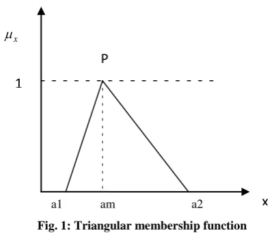
i.e. three values a1,am, and a2 represents a triangular number
denoted by
~
1 2
( , m, ) A a a a
[image:2.595.318.519.78.248.2]
Fig. 1: Triangular membership function
The above figure shows the triangular membership function of a fuzzy set
~
P,
~
P=(a1, am, a2). The membership value reaches the
highest point at ‘am’, while ‘a1’ and ‘a2’ denote the lower bound
and upper bound of the set
~
Prespectively.
2.2. Fuzzy Arithmetic Operations
Let
~
1 2 3
( , , ) A a a a and
~
1 2 3
( , , )
B b b b be the two triangular fuzzy numbers, the four basic operations that can be performed on triangular fuzzy numbers are as follows:
1. Addition:
~ ~
1 1 2 2 3 3
( , , )
A B a b a b a b 2. Subtraction:
~ ~
1 1 2 2 3 3
( , , )
A B a b a b a b .
This subtraction operation exist only if the following condition is satisfied DP(A) ≥ DP(B), where DP A( )~ (a3a1) / 2and
~
3 1
( ) ( ) / 2
DP B b b ,where DP denotes difference point of a triangular fuzzy number.
else,
~ ~
1 3 2 2 3 1
( , , )
A B a b a b a b 3 .Multiplication:
~ ~
1 2 2 1 2 2, 2 2, 2 3 3 2 2 2
A B a b a ba b a b a b a b a b
4. Division:
~ ~
1 2 3
1 3 2 1 3
~ ~
2 2
/ , , ; provided
and are all non zero numbers.
a a a
A B
b b b b b
A B
3.
FUZZY BISERIAL QUEUES
According to Zadeh development theory [1978] and by the use of the possibility theory concepts, fuzzy Markov chain [1982], Li and Lee [1989] proposed that every fuzzy queuing model could be considered as a classical queuing theory model by considering following changes: the probability distribution function of the time between two consecutive arrivals which is assumed to follow the exponential distribution with the parameter is considered to be
~
in fuzzy environment which is an approximation of the mean of its possibility distribution and similarly, the servicing rate is considered to be the fuzzy number
~
which is the mean of its possibility distribution in fuzzy environment. The following notation has been used throughout the course of the present paper:
x
x
1
P
: Fuzzy arrival rate
: Fuzzy service raten
: Number of customers / jobs arriving~
( )
ij
P s : Possibility that the system is in the state (i, j) at any time t
L
: Mean queue length of the customers system ( )E W : Expected waiting time customers (jobs)
~
S
L : Fuzzy mean queue length (number of customers) of the system
~
( S)
E W : Expected fuzzy waiting time of the system
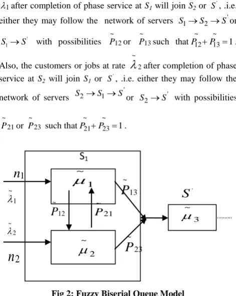
3.1. Mathematical Model
The fuzzy biserial queue model is comprised of two servers Sand
'
S. The server S consists of two biserial service servers S1 and
S2. The service server
'
Sis commonly linked in series with each of the two parallel biserial servers S1 and S2. Let there be n1, n2
number of customers arriving at the servers S1 and S2 with fuzzy
arrival rates
~ ~
1 and 2
. Let
~ ~
1 and 2
be the fuzzy service rate at servers S1 and S2 and
~ 3
be at server '
S. Queues Q1, Q2, Q3 are
said to be formed in front of the service servers S1, S2 and
server '
S, if they are busy. Customers or jobs arriving at rate
~ 1
after completion of phase service at S1 will join S2 or S', .i.e.
either they may follow the network of servers S1S2S'or
' 1
S S with possibilities
~ 12
P or
~ 13
P such that
~ ~
12 13 1
P P . Also, the customers or jobs at rate
~ 2
after completion of phase service at S2 will join S1 or'
S, .i.e. either they may follow the network of servers
'
2 1
S S S
or S2S' with possibilities ~
21
P or
~ 23
P such that
~ ~
21 23 1
P P .
[image:3.595.55.291.369.665.2]Fig 2: Fuzzy Biserial Queue Model
The system characteristic of interest is the average queue length and the expected waiting time of customers / jobs .From the knowledge of queue theory as given by Vinod et al [2006], if
1 2 21
1 12 21
( ) 1
1 p i
p p
,
2 1 12
2 12 21
( ) 1
1 p ii
p p
and,
13 1 2 21 23 2 1 12 3 12 21
( ) 1
1
p p p p
iii
p p
,
then ,the average queue length and the expected number of customers for a crisp biserial queuing system are given by
Mean queue length = 1 2 3 1 2 3
1 2 3
1 1 1
L L L L
Where, 1 1 2 2 3 3
1 2 3
, ,
1 1 1
L L L
,
1 2 21
1
1 1 12 21
p p p
,
2 1 12
2
2 1 12 21
p p p
,
13 1 2 21 23 2 1 12 3
2 1 12 21
p p p p
p p
and
Expected waiting time =E w( ) L
, where 1 2.
The model finds its applications in manufacturing or assembling line process in which units processed through a series of stations, each performing a given task. Practical situation can be observed in a registration process (vehicle registration) where the registrants have to visit a series of desks (advisor, department chairperson, cashier, etc.), or in a clinical physical test procedure where the patients have to pass through a series of stages (lab tests, electrocardiogram, chest X-ray etc.). The customers or items after getting service at stage S1 may join the service S2 or
may directly avail the service
S
'. Similarly, the customers or items after getting service at stage S2 may join the service S1 ormay directly avail the service
S
'.In classical queuing theory, arrival rates and service times are required to follow certain probability distribution. In the present paper, we study the proposed biserial queue model in fuzzy environment.
3.2
Solution Methodology
The system data which are gathered from the real world problems always has a sort of ambiguity. The “fuzzy set” is a tool to consider these ambiguities. On the other hand, to determine the parameters of the model in the real world, generally, the expert ideas or sampling data can be used. It can be claimed that there is a sort of ambiguity in the both mentioned methods. In the first case, the ambiguity is due to the lack of the preciseness and enough specialty. In the second case, the ambiguity is due to the lack of enough sampling data. Because of this ambiguity, in this paper, it is preferred to use the fuzzy parameters instead of the certain ones for the suggested queue model. To estimate a parameter as a fuzzy number and to change the input data (Arrival rate, Service rate) into the fuzzy numbers, the method of Buckley and Qu method [1990] is used.
Since the arrival rate (
~
), service rate (
~
) are not known precisely, therefore, we use triangular fuzzy numbers to represent them.
Let
~ ~
1, 2, 3 , 1, 2, 3
Where 1 2 3, 123 based on subjective judgment. The membership of ~ ~
~ ~
and
are defined as follows:
S
1'
S
~12
P
P
~21~ 1
~ 2
1
n
2
n
~ 3
~ 13
P
~ 23
P
~1
~ 2
~ 1 1 1 2 ~ 2 1 3 2 3 3 2 3 0 0 if if if if ~ 1 1 1 2 ~ 2 1 3 2 3 3 2 3 0 0 if if if if
Using the concept of - cut method, we have
~ ~ 12 1 1
2 1
~
~ 3
3 3 2
3 2
2 1 1 3 3 2
~
~ 1
2 1 1
2 1
~
~ 3
3 3 2
3 2
2 1 1 3 3 2
, ,
~ ~ 12 1 1
2 1
~
~ 3
3 3 2
3 2
2 1 1, 3 3 2
p p
p p p p
p p
p p
p p p p
p p
p p p p p p p
Let the fuzzy arrival rates
~ 1
,
~ 2
; fuzzy service rate
~ ~ ~ 1, 2, 3
and various fuzzy possibilities
~ ~ ~ ~
12, 13, 21, 23
p p p p are defined as
~ ~
1 2 3 1 2 3
, , , , ,
i i i i i i i i
and
~
1 2 3
, ,
ij ij ij ij
p p p p for
various values of i & j.
Therefore, i
i21i
1i, i3
i3i2
i
i2i1
1i, i3
i3i2
pij
pij2p1ij
p1ij,p3ij
pij3pij2
Since , 1 1
1 2 21
1 1 12 21
1
1
p
L
p p
, therefore
1 1 2 21
1
1 1 12 21
1 1 p L p p
2 1 1
2 2 2
2 1 1
1 1 1
2 1 1
21 21 21 1 2 21
3 3 2
2 2 2
3 3 2
1 1 1
3 3 2
21 21 21
,
.
p p p
p
p p p
2 1 1
1 1 1
2 1 1
12 12 12
2 1 1
21 21 21
1 12 21
3 3 2
1 1 1
3 3 2
12 12 12
3 3 2
21 21 21
1
,
1
1
p p p
p p p
p p
p p p
p p p
3 3 2
12 12 12
3 3 2
1 1 1
3 3 2
21 21 21
1 12 21
2 1 1
12 12 12
2 1 1
1 1 1
2 1 1
21 21 21
1 , 1 1 1 1 1
p p p
p p p
p p
p p p
p p p
Therefore,
1 2 21
1
1
1
12 21p
L
p
p
2 1 1
2 2 2
2 1 1
1 1 1
2 1 1
21 21 21
3 3 2
12 12 12
3 3 2
1 1 1
3 3 2
21 21 21
3 3 2
2 2 2
3 3 2
1 1 1
3 3 2
21 21 21
2 1 1
12 12 12
2 1 1
1 1 1
2 1 1
21 21 21
, 1
1
p p p
p p p
p p p
p p p
p p p
p p p
On taking 0 and 1in the above, we obtain an approximate triangular fuzzy number. Thus
1 1 1 3 3 3
1 2 21 1 2 21
3 3 3 1 1 2
~ 12 21 1 12 21 1 1 2 3
1 2 2 2 1 1 1
1 2 21
2 2 2
12 21 1
,
,
1
1
,
,
1
p
p
p p
p p
L
L L L
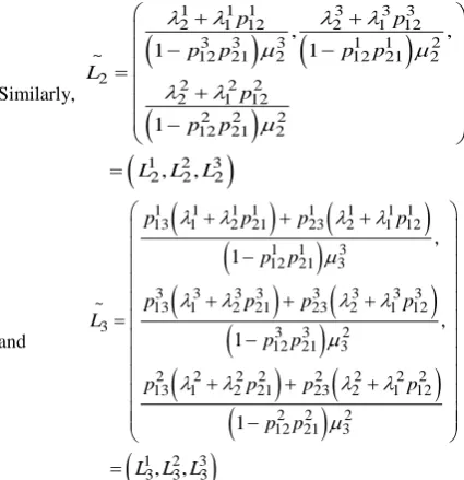
Similarly,
1 1 1 3 3 3
2 1 12 2 1 12
3 3 3 1 1 2
~ 12 21 2 12 21 2
2 2 2 2
2 1 12
2 2 2
12 21 2 1 2 3
2 2 2
, ,
1 1
1
, ,
p p
p p p p
L
p
p p
L L L
and
1 1 1 1 1 1 1 1
13 1 2 21 23 2 1 12
1 1 3
12 21 3
3 3 3 3 3 3 3 3
~ 13 1 2 21 23 2 1 12
3 3 3 2
12 21 3
2 2 2 2 2 2 2 2
13 1 2 21 23 2 1 12
2 2 2
12 21 3 1 2 3
3 3 3
, 1 , 1 1 , ,
p p p p
p p
p p p p
L
p p
p p p p
p p L L L
Therefore, Average (mean) fuzzy queue length
~ ~ ~ ~
1 2 3 1 2 3 1 2 3
1 2 3 1 1 1 2 2 2 3 3 3
1 1 1 2 2 2 3 3 3
1 2 3 3 3 3 1 2 3 1 2 3
, , , , , ,
, , , ,
L L L L L L L L L L L L L
L L L L L L L L L l l l
Also,
~ ~ ~
1 2 3 1 2 3
1 2 1 1 1 2 2 2
1 1 2 2 3 3
1 2 1 2 1 2 1 2 3
( , , ) ( , , ) , , , ,
The fuzzy average waiting time of the customers / jobs is
~ ~
1 2 3 ~
1 2 3
3
1 2
1 2 3
1 3 2 1 3
, , , , 2 2
, , , ,
l l l L
E W
l
l l
w w w
Therefore, the membership functions for
~
Land
~
E W
are
~ 1 1 1 2 2 1 3 2 3 3 2 3 0
0 L L
if L l L l
if l L l l l
l L
if l L l l l if l ~ 1 1 1 2 2 1 3 2 3 3 2 3
0 W
w
w
0 W W
if w W w
if W w w w
w W
if W w w w if w
Since the system characteristics are described by membership function, it preserves the fuzziness of input information. However, the designer would prefer one crisp value for one of the system characteristics rather than fuzzy set. In order to overcome this problem we defuzzify the fuzzy values of system characteristic by using the Yager’s [1981] formula crisp
1 2 2 3
4
a a a
A if
~
1, 2, 3
A a a a .
4.
NUMERICAL ILLUSTRATION
Consider nine customers/jobs are processed through the network of queues Q1, Q2 and Q3 with the servers S1, S2 andS'. The
servers S1 and S2 are parallel biserial servers and server S'linked
in series with each of two servers S1 and S2. The number of the
[image:5.595.55.268.74.294.2]customers, fuzzy mean arrival rate, fuzzy mean service rate and various associated possibilities are given as in Table 1.
Table 1: Input variable of the proposed biserial queue model
Arrival Rate
Service Rate
Possibilities
n1=5
~
1 (5,6,7)
~1(12,14,16)
~
12 (.6,.7,.8)
p
n2=4 ~
2 (4,5,6)
~2(14,15,16)
~
13 (.4,.3,.2)
p
~
3 (9,12,15)
p~21(.3,.5,.6) ~
23 (.7,.5,.4)
p
Our aim is to find the expected waiting time and average queue length of customers/jobs.
Here, we have
~ ~ 1 2 ~ 30.7452,0.9233,0.9341 , 0.8413,0.9431,0.9436 and 0.9461,0.6867,0.7542
L L
L
Therefore, mean (average) queue length of customers
~ ~ ~ ~
1 2 3 2.5326, 2.5531, 2.6319
L L L L
Also,
~ ~ ~
1 2 9,11,13
Therefore, the expected waiting time of the customers
~ ~ 3 1 2 ~1 3 2 1 3
2 2
, ,
0.2302, 0.2321, 0.2393 l
L l l
E W
On, defuzzify, we getE( ) 11, E w( )0.233425
[image:5.595.317.484.565.715.2]2.520 2.54 2.56 2.58 2.6 2.62 2.64 2.66 0.1 0.2 0.3 0.4 0.5 0.6 0.7 0.8 0.9 1
Figure 3 : Expected fuzzy mean queue length
~
E L
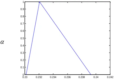
0.230 0.232 0.234 0.236 0.238 0.24 0.242 0.1
[image:6.595.57.259.81.225.2]0.2 0.3 0.4 0.5 0.6 0.7 0.8 0.9 1
Figure 4 : Expected fuzzy waiting time
It indicates that the support of
~
E W
ranges from 0.2302 to
0.2393, .i.e. the expected waiting time is fuzzy, it is impossible for its values to fall below 0.2302 or exceed 0.2393. The
-cut at
1
is exactly 0.2321, which is the most possible value for the expected waiting time in the system.Similarly, the mean queue length of customers (jobs) in the system falls between 2.5326 and 2.6319. It indicates that the mean queue length of customers in the system will never exceed 2.6319 or fall below 2.5326. The most possible mean queue length of customers (jobs) is 2.5531.
5.
CONCLUSION
In this paper, the characteristic of biserial queuing system in fuzzy environment has been studied. Considering arrival rate, service rate are fuzzy, the expected waiting time and mean queue length of customers have been computed using fuzzy arithmetic operations. In the literature, the various system characteristics are assumed to be exact, but in real practical life the input information are almost uncertain, imprecise, and incomplete. The proposed fuzzy biserial model is more suitable for designer and practitioner since it deals with incomplete information. Fuzzy triangular membership function, -cut approach and fuzzy arithmetic operations are used to construct system characteristic membership function. The study may further be extended by introducing more parallel, biserial servers and by introducing concept of linkage network of proposed biserial model with a system of parallel machines in series under fuzzy environment.
6.
ACKNOWLEDGEMENT
The authors would like to thanks anonymous referees and editor of the journal for their constructive comments which has improved the quality and presentation of this paper.
7.
REFERENCES
[1] Brak, S., and Fallahnezhad, M.S. 2012. Cost analysis of fuzzy queuing system. International Journal of Applied Operational research, 2(2), 25-36.
[2] Buckley, J.J. 1990. Elementary queuing theory based on possibility theory. Fuzzy Sets and Systems, 37, 43-52. [3] Buckley, J.J., and Qu, Y. 1990. On using cuts to evaluate
fuzzy equations. Fuzzy Sets and Systems, 38, 309-312. [4] Finch, P.D., 1960 . On transient behaviour of simple queue.
J. Roy Statst, Soc., 22, 277-283.
[5] Jackson, R.R.P. 1954. Queuing systems with phase-type service. Operational Research Quarterly, 5, 109-120. [6] Kao, C., Li, C., and Chen, S. 1999. Parametric
programming to the analysis of fuzzy queues. Fuzzy Sets and Systems, 107, 93-100.
[7] Kumar, V., Singh, T.P., and Kumar, R. 2006. Steady state behaviour of a queue model comprised of two subsystems with biserial channels linked with a common channel. Ref Des Era JSM, 1(2), 135-152.
[8] Li, R.J., and Lee, E.S. 1989. Analysis of fuzzy queues. Computers and Mathematics with Applications, 17(7), 1143-1147.
[9] Little John, D.C. 1965. A proof of queuing formula:
"
L
w
"
. Operation Research, 13, 400-412.[10] Maggu, P.L. 1970. Phase type service queues with two servers in biseries. Journal of Operational Research Society of Japan, 13(1), 1-6.
[11] Nagoorgani, A., and Retha, W. 2006. Fuzzy tandem queues. Acta Cienicia Indica. XXXII(M), 257-263.
[12] Negi, D.S., and Lee, E.S. 1992. Analysis and simulation of fuzzy queues, Fuzzy Sets and Systems, 46, 321-330. [13] Parbhu, N.U. 1967. Transient behaviour of tandem queues.
Management sciences, 13, 631-639.
[14] Prade, H.M. 1980. An outline of fuzzy or possiblistic models for queuing systems, in: P.P Wang, S.K. Chang (Eds.), Fuzzy Sets: Theory and Applications to Policy Analysis and Information Systems. Plenum Press, NewYork, 147-153. [15] Pourdarvish, A, and Jamshidi, Y. 2008. Application of fuzzy
set in transient behaviour of queuing system. JISSOR, XXIX.
[16] Reich, E. 1957. Waiting times when queues are tandem. Ann. Maths Statist, 28(3), 728-733.
[17] Robert, L., and Ritha, W. 2010. Machine interference problem with fuzzy environment. I. J. Contemporary Math. Science, 5(39), 1905-1912.
[18] Ritha, W., and Robert, L. 2009. Application of fuzzy set5 theory to retrial queues. International Journal of Algorithms, Computing and Mathematics, 2(4), 9-18.
[19] Singh, M. 1979. On certain queuing networks of serial/bi-serial channels. Ph.D Thesis, Meerut University, Merrut. [20] Singh, T.P. 1986. On some networks of queuing and
scheduling system. Ph.D. Thesis, Garhwal University, Srinagar, Garhwal.
[21] Singh, T.P., Kumar, V., and Kumar, R. 2005. On transient behaviour of queuing network with parallel biserial queues. JMASS, 1(2), 68-75.
[22] Singh, T.P., and Pardeep 2009. Serail queue model with blocking under fuzzy environment. JMASS, 5(2), 86-94. [23] Singh, T.P., and Kusum, 2011. Trapezoidal fuzzy network
queue model with blocking. ABJMI, 3(1), 185-192.
[24] Stanford, R.E. 1982. The set of limiting distributions for a Markov chain with fuzzy transition probabilities. Fuzzy Sets and Systems, 7, 71-78.
[25] Suzuki, T. 1963. Two queues in series. Journal of Operational Research Society of Japan, 5, 149-155.
~
E W
[26] Yager, R.R. 1981. A procedure for ordering fuzzy subsets of the unit interval, Inform. Sci. 24, 143-161.
[27] Zadeh, L. A. 1978. Fuzzy sets as a basis for a theory of possibility. Fuzzy Sets and Systems, 1, 3-28.
[28] Zimmermann, H.J. 1995. Fuzzy set theory and its applications, second ed., Kluwer Academic Boston.
[29] Zhang, R., Phillis, Y.A., and Kauilkoglou, V.S. 2006. Fuzzy Control of Queuing Systems. ISBN 1852338245, Springer Verlags.