Edge Extraction Algorithm using Linear Prediction Model on Dental X ray Images

Edge Extraction Algorithm using Linear Prediction

Model on Dental X-ray Images

Gayathri V

Dept. of CSE Amrita Viswa Vidyapeetham

Tamil Nadu

Hema P Menon

Dept. of CSE Amrita Viswa Vidyapeetham

Tamil Nadu

K A Narayanankutty

Dept. of ECE Amrita Viswa Vidyapeetham

Tamil Nadu

ABSTRACT

This paper focuses edge extraction from dental x-ray images for the root canal procedure, using the linear prediction (LP). The major issues of processing the dental X-ray images are caused due to the misalignment and the variation in the contrast, by the very modality of acquisition. Also the differences in the shapes and orientations of the teeth pose yet another difficulty in the processing. Thus, in order to overcome these challenges, the LP residual based approach is used in this paper to obtain better root canal edge information. In the present work, the input image is processed by the 10th

order LP method to obtain LP residual image. The LP residual of the input image is found to provide better edges as compared to the conventional methods. Also the edge map obtained by the LP method is compared with previous work [7] on zero frequency resonator (ZFR) based edge extraction and is found to give a better edge map. Effectiveness of the LP residual method is confirmed by the visual inspection of the edge map and also from the subjective evaluation.

General Terms

Edge extraction algorithms, root canal length calculation

Keywords

Edge extraction, dental x-ray image, linear prediction model, zero frequency resonators

1.

INTRODUCTION

The human teeth are of various structures, namely those with single root (incisors), double roots (pre-molars) and triple roots (molars). The root canal edges are required in many treatments and analysis of teeth, like the root canal treatment where the root length is a necessary parameter of the treatment process. The quality of the edge map obtained over non-uniform dental x-ray images by using the conventional edge extraction techniques is discussed and analyzed in our previous work [7]. The analysis obtained from paper [7] indicates the necessity for a better and efficient edge extraction method which generates less spurious edges. The edge extraction of dental x-ray images is one of the stages required in processing and analyzing dental x-ray images. Thus the accuracy of the edge extraction stands as a necessary phase in most of the x-ray analysis and can affect the later stages of processing, mainly while finding the root canal depth and length.

Researches in the field of dental x-ray images are very few. For perfectly aligned and uniform x-ray images, conventional edge extraction techniques have been used in the paper [1]. The basic binarization technique is to extract the edges from single tooth x-ray images in the paper [2]. In case of perfectly aligned tooth x-rays, morphological operations are used as the pre-processing step to obtain the root in the paper [3]. Zero

Frequency Resonator (ZFR) filter is an advanced method for edge extraction [4]. This ZFR filter method has been implemented in our previous work [7] on dental x-ray images. The ZFR filter extracts the impulse-like discontinuities from the x-ray image, thereby resulting in the extraction of the edges. It is assumed that the energy of the signal is distributed uniformly around all the frequencies present in the signal including the zero frequency. Therefore, the impulse-like discontinuities of the signal can be obtained by filtering the x-ray image by implementing cascade of two resonators located on the zero frequency. Later, the edges are obtained by performing trend removal operation over the filtered signal by the use of Laplacian operator. Also another method for obtaining the discontinuities is by the linear prediction analysis [5]. LP analysis is based upon the concept of prediction of the current signal values using the past signal samples. Generally, LP analysis is used for one-dimensional signals. The paper [6] proposed by James Z. Zhang, Peter C. Tay, Robert D. Adams implements the LP residual analysis over the standard gray scale images and is found to generate better edge maps. The present work is therefore carried out in this direction. In this work, thus, the linear prediction (LP) residual images are used as the edge map, for the root canal edge extraction is highlighted.

model plays a crucial role in the computation of the edge map. The resultant edge map may be “thick” or “broken lines” when a threshold is applied on the gradient magnitude after diffusion. These issues were addressed by adding constraints in the PDE model to improve the edge thinning and connectivity [10]. A drawback of the diffusion based methods is that they are computationally expensive. Typically, a large number of iterative steps are required to obtain a high quality edge map. Multi-resolution schemes are employed to reduce the computational load [20]. But these approaches often create artifacts such as blotches (false regions) and staircases (false step edges) in the edge map. All the smoothing operations can be interpreted as a lowpass filtering, thus reducing the effect of the high-frequency components of the image. Since rapid changes in the image pixels are associated with an edge, the edge information is extracted using this principle linked edge information with the high-frequency information. Hence, the edge extraction and smoothing operation are contradictory, in the sense that edge extraction involves difference operation highlighting the high-frequency components, and smoothing operation highlights the low-frequency components.

LP is a popular technique which is widely used in speech and audio signals for extracting some useful information like pitch, resonances etc. The basic idea behind the LP is to predict the current sample value in a signal based on the past P sample values, where P is the order of prediction. Based on this idea, the LP analysis is all about estimating P linear prediction coefficients (LPCs) which best fits the given data. The difference between the predicted signal and the actual signal is known as the linear prediction error or popularly known as the linear prediction residual. In one-dimensional case, the LP residual captures the sharp variations in the signal. This work exploits the very nature of LP residual in extracting such sharp variations in dental x-ray images. These are some works done in this direction by exploiting the nature of the residual in images [2].

The organization of the paper is as follows: Section 2 discusses the implementation details using the linear prediction model. Section 3 contains the subjective analysis obtained for the linear prediction as well as the ZFR based method for obtaining the edge map. The summary and conclusion is included in Section 4.

2.

IMPLEMENTATION DETAILS

2.1

Data Set Details

40 digital dental x-ray images have been used to conduct the experiment. The x-ray images include teeth which contain single, double and triple roots. Also it contains x-ray images of teeth belonging to both the upper as well as the lower jaw. The x-ray images are acquired using Kodak RVG 5100 device. The x-ray image of the required tooth is captured by placing the x-ray equipment over the tooth region and thereby resulting in images which are of different orientations. This poses a great challenge in identifying the root canal edge map. Traditionally, Linear Prediction is used to predict future values of a signal using past values. The goal is to minimize prediction errors. In this algorithm, we a novel method of utilizing prediction errors to extract edges of images is proposed. In this method, smooth prediction errors are minimized while steep changes (larger errors) are amplified. Therefore, when applied to image edge detection, edge information can be accurately extracted [4].

2.2

System Design

Input Image

2.3

Pre-Processing

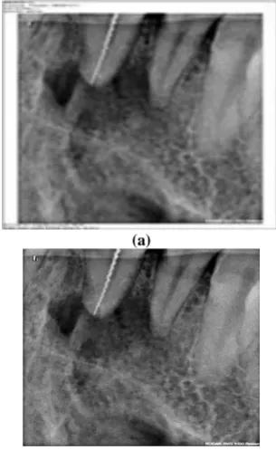
The presence of a border noise can be seen in all the dental x-ray images used in this paper. Therefore, as a pre-processing noise removal step, the border noise is removed from the images. For the removal of such border noise, the projection profile technique is used. The projection profiles, both the horizontal projection profile and the vertical projection profile are used to obtain the locations of the horizontal and vertical borders respectively. Finally, the border noise is removed after locating their pixel positions. Thereby, generating border noise removed x-ray image. The Fig. 1(a) shows the original image and Fig. 1(b) gives the border-noise removed x-ray image.

(a)

(b)

Fig 1: Dental X-Ray image (a)Original Image (b) The border noise removed image

Obtain Linear Prediction Edge Map

Post Processing Border Noise Removal

2.4

Linear Prediction Analysis for Edge

Detection

Linear prediction has been widely used in estimating future

values of a signal based on past values. Let x n   be the estimated value, x[n−k] be the past values. A one-step forward linear predictor of order p can be expressed as follows:

1

( ) p

p k

x n a k x n k



 _{  } 

 



Where, ap( )k

are prediction coefficients.

Let fp[n] be the prediction error. fp[n] can be expressed as:

0

[ ]

[ ]

( )

p

p p

k

f

n

x n

x n

a

k x n k



 





_{ }







The MMSE of fp[n] can be expressed as: 2

0

min{ } min{ [ [ ] ]} (0) ( ) ( ) p

f

p p xx

p xx

k

e E f n r a k r k



  



where rxx(−k) is the conjugate of the

th

k _{autocorrelation} value of x[n].

LP achieves its accuracy of predicting future values of a signal by minimizing errors. However, when there are steep changes in a signal, LP cannot track the changes accurately and therefore causes larger errors at discontinuities than those areas with gradual changes in that signal. Because image edges are steep changes in intensity at adjacent pixels (locality), larger errors exist between the original image and the predicted image at those local discontinuities. Consequently, the “shortcoming” of LP provides an opportunity to detect image edges if these errors can be amplified and extracted.

2.4.1

Algorithm

Suppose we have an image I, its edge information can be detected using LP as follows which has been proposed by taking inputs from paper [4]:

Step 1:-

Apply LP on each row along +x direction to generate a predicted image Ix _{and along −x direction to generate a}

predicted image Ix _{. The edge information along}

x-direction (the amplified errors) can be obtained by:

, x x

x error

I



I



I

Step 2:-

Apply LP on each row along +y direction to generate a

predicted image Iy_{and along} −y _{direction to generate a} predicted image Iy_{. The edge information along y-direction}

(the amplified errors) can be obtained by:

,

y

y

y error

I



I

_



I

_

Step 3:-

The edges of the image are contained in (similar to a “gradient map”):



2

2



,

,

x error

y error

edgetrial

I



I



I

Step 4:-

Also obtain the intensity range Irange[] of the root canal edge

using automatic histogram method. If the Iedgetrial fall under the

intensity range obtained in Irange[], then, take that Iedgetrial as

Iedge.

Step 5:-

Set appropriate threshold to extract the edge map.

(a)

(b)

(d)

(e)

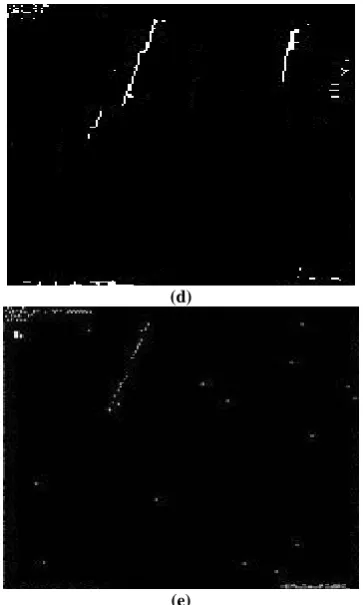
Fig.2: Dental x-ray images (a) Original image (b) edge map obtained by applying LP algorithm without considering the Irange[] (c) LP edge map obtained by

considering the Irange[] (d) LP edge map obtained after

post-processing(e) edge map obtained using ZFR filter based method

2.5

Post Processing

It can be seen from Fig.2 (b) and Fig.2(c) that even though the edges are more prominent than the edges obtained using ZFR based method shown in Fig.2(e), the obtained edges have gaps in between. Therefore, it can be said that the edge pixels are not continuous. Therefore, an adaptive edge linking algorithm is used to obtain continuous edges. The ON pixels are scanned in a raster scan manner and its neighbouring pixels are checked, if there exists another ON pixel in its neighbourhood, then the algorithm is scanned in that direction till the last ON pixel is encountered and turning on the OFF pixels through the scan. Else, if there is no ON pixel in the neighbourhood, the gap is checked. If the gap < thresholdgap,

then the gap pixels are turned ON else, the gap pixels are left unchanged. The Fig.2(d) shows the edge linked result of the original image used in Fig.2(a). Fig 2(d) shows the edge map after performing the edge linking algorithm used in the post processing stage and also Fig 2(e) shows the result obtained using the ZFR based method.

2.6

Root Length Calculation

From the obtained edge map, the root length in terms of number of pixels can be calculated. The root length is needed for the dentist during procedures like root canal treatment where the root length is needed to identify the quantity of the filling. Generally, dentists use manual exertion of pins of various lengths into the root canal cavity to identify the root length. The automated root length calculation relieves the patient the painful process of inserting pins. This automated root length calculation also helps dentist from the time consuming step of root length calculation.

2.6.1

Connected Component Analysis

Connected component analysis is used in this paper to calculate the root length. The edge map of the digital dental x-ray image is analysed for the presence of any connected components. The count of the connected component gives the number of roots present in the edge map and the starting and ending pixel location of each of the obtained connected components give the starting and ending co-ordinate locations of each of the connected components. Once the start and end points are obtained, the distance can be calculated using the Euclidian distance formula as given below,

2 2

( 2

1)

( 2

1)

d



x



x



y



y

The distance d will give the count of the pixels present in the root canal edge.

Table 1. Root Length Table

Figure

Root Length (No. of Pixels)

Fig 1(a) 107.32

3.

RESULT ANALYSIS

3.1 Subjective Analysis

Forty subjects, including experts participated in the subjective evaluation. The stimuli for the subjective test are generated using ZFR filters and LP edge extraction algorithm on 30 dental x-ray images. The subjects were asked to visually compare the detected edges in the obtained edge maps. Also, subjects were asked to provide their opinion scores in a five point scale. The justification of each scale is given in Table 2.The filenames of each of these edge maps are encoded to avoid bias towards any particular method. After obtaining the opinion scores for each edge maps, the mean of the opinion score are computed across all subjects for each method. These mean opinion scores (MOS) are presented in Table 3.

Table 2: Justification of the scales used for MOS

Rating Quality of the

obtained root edge

Justification

1 Very Poor No root canal edge detection

2 Poor Broken root canal edges

3 Good Marginally good root

canal edge detection

4 Very Good Almost all root canal edges are detected 5 Excellent Exact root canal edges

Table 3: MOS obtained for each method in the subjective evaluation

Method ZFR LP

MOS 3.1 3.8

based method, the quality of the same has to be further improved for obtaining more efficient edge maps.

3.2 Objective Analysis

The edge extraction algorithm can be evaluated objectively with the assumption that, ideally, when the edge extraction is exact, there will be only one connected component and the length of the connected component will be large. Thus, the count of connected components and the count of pixels in the biggest connected component are identified from the edge map. The edge extraction technique which gives the minimum number of connected components with the largest number of pixels in the connected component is assumed to be a better edge extraction technique.

To conduct the objective evaluation of the edge detectors, the same 40 dental x-ray images which were used for the subjective evaluation have been used. The average of the count of the connected components obtained for each of the edge detection method as well as the average of the largest connected component is calculated. The average values thus obtained for each of the edge detectors are given in the table 4 below.

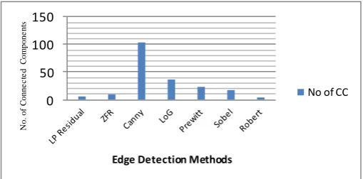
Table 4: Table for objective evaluation of edge detectors

Method Average Number of

Connected Components

Average Pixel count of the largest connected component

Robert 4.109 12.432

Sobel 16.456 32.410

Prewitt 22.621 45.785

LoG 37.420 110.70

Canny 103.364 102.537

ZFR 9.312 117.140

LP Residue 6.71 133.831

From table 4, it can be observed that lp residue based edge extraction technique gives the minimum number of connected components as well as the largest connected components as compared to the other edge extraction techniques. It can be noted that the length of the largest connected component is similar in case of LoG and ZFR filter based edge extraction method, but, the count of the connected components is larger in case of LoG than that of ZFR which implies that ZFR filter gives better noise localized edge map than LoG. The Canny edge extraction method gives fairly good results with respect to the length of the largest connected component, but, due to its over segmentation, the cont of the connected components obtained is very high, which makes it undesirable to obtain edge map in case of dental x-ray images. The values obtained for the objective analysis are diagrammatically represented in Fig.3 and Fig.4.

0 50 100 150

N

o. of

C

on

ne

c

te

d C

om

po

ne

nt

s

Edge Detection Methods

No of CC

Fig 3: Plot of connected components obtained for each edge detection methods

0 50 100 150

N

u

m

b

e

r o

f P

ix

e

ls

Edge Detection Methods

Avg Pixel Count

Fig 4: Plot of average count of connected components obtained for each edge detection methods

3.3 Accuracy of Tooth Classification

40 digital dental x-ray images have been used for determining the accuracy of the tooth structure classification algorithm. The dental x-rays considered contains images which have uniform tooth, misaligned tooth, tooth with decays and tooth with fillings. The classification algorithm is applied to each of such dental x-ray images and the correctness of classification is noted. The accuracy is calculated as follows:

The observation is given in table 5.

Table 5:Table of accuracy calculation of tooth structure analysis

Count of correctly classified dental x-ray images

33

Count of correctly

misclassified dental x-ray images

7

Accuracy 82.5%

4.

SUMMARY AND CONCLUSION

edges obtained by using ZFR filter method. From the analysis it can be concluded that the linear prediction residue based algorithm gives better edge maps as compared to the ZFR filter method in the case of non-uniform digital dental x-ray images. The experiments reveal that LP residual gives better results for most of the images in the dataset. This is confirmed using both the subjective and objective evaluation. Also the root canal length in terms of number of connected components and Euclidian distance are calculated which is very useful in case of root canal treatment. The automatic tooth structure identification is conducted based on the number of roots and the system achieves 82.5% accuracy. Hence the use of linear prediction model is suggested as the best method for root canal edge extraction from misaligned teeth in digital dental x-ray images and that the number of connected components in the edge map can be taken as a good measure for assessing the accuracy of the edge extraction method being used. This work could be further extended to analyze the complete structure of the tooth.

5.

ACKNOWLEDGMENT

The authors sincerely thank Dr.Premkumar, Dental Health Care Clinic, Thrissur for providing necessary guidance throughout the work. The authors would also like to thank Amrita Viswa Vidyapeetham for having provided the required resources in the Amrita – Cognizant Innovation Lab for carrying out the research work.

6.

REFERENCES

[1] Azam Amini Harandi, Hossein Pourghassem, “A Semi Automatic Algorithm Based on Morphology Features for Measuring of Root Canal Length”, in Pro IEEE International Conference on Communication Software and Networks(ICCSN), 2011.

[2] S. Oprea, C. Marinescu, I. Lita, M . .Iurianu, D. A. Visan, I. B. Cioc, "Image processing techniques used for dental xray image analysis," in Proc. Electronic Technology 2008 ,pp. 125-129,2008.

[3] Balázs Benyó, László Szilágyi, Tamás Haidegger, Levente Kovács, and Csaba Nagy-Dobó, "Detection of the Root Canal’s Centerline from Dental Micro-CT Records", in proc.31st Annual International Conference of the IEEE EMBS Minneapolis, Minnesota, USA, 2009. [4] Anil Kumar Sao B, Yegnanarayana 2012 “Edge Extraction Using Zero-Frequency Resonator “, in proc. Springer,Signal Image and Video Processing, Volume 6, Issue 2, pp 287-300.

[5] Makhoul, J , “Linear Prediction: A Tutorial Review", in proc. Proceedings of the IEEE, Vol. 63, Issue 4, 561-580,1975.

[6] James Z. Zhang, Peter C. Tay, Robert D. Adams 2010 " A Novel Image Edge Detection Method Using Linear Prediction", in Proc.Circuits and Systems (MWSCAS), 53rd IEEE International Midwest Symposium, 620 – 623,2010.

[7] Gayathri V, Hema P Menon , "Root Canal Edge Extraction Using Zero Frequency Resonance Filter in Dental X-Ray Images", accepted in International Conference on Speech Signal Processing (ICSSP), 2014. [8] O. Nomir, M. A Motataleb," Hierarchical dental x-ray

radiographs matching," in Proc. ICIP, pp. 2677-2680, 2006.

[9] O. Nomir, M. A Motataleb, "Human identification from dental x-ray images based on the shape and Appearance of the teeth," IEEE Transactions on information forensics and security, vol. 2, Issue. 2, pp. 188-197.2007.

[10]O. Nomir, M. A Motataleb, "Combining matching algorithms for human identification using dental x-ray radiographs,"in Proc. ICIP, vol 2, 2007

[11]Roberts,L.G .”Machine Perception of Three-Dimentional Solids”, in Optical and Electro-Optical Information Processing, Tippet, J.T.(ed.), MIT Press, Cambridge, Mass, 1965.

[12]Sobel,I.E, ”Camera Models and Machine Perception,”Ph.D. dissertation, Stanford University, Palo Alto, Calif, 1970.

[13]Prewitt,J.M.S, “Object Enhancement and Extraction”, in Picture Processing and Psychopictorics, Lipkin, B.S., and Rosenfeld, A.(eds.), Academic Press, New York, 1970. [14]S. Kiattisin, A Leelasantitham, K. Chamnongthai, K.

Higuchi, "Amatch of x-ray teeth films using image processing based on special features of teeth," in Proc. Signals Annual Conference, Vol.1, pp. 35-39, April 2008.

[15]Canny,J., “ A Computational Approach for Edge Detection”, IEEE Trans. Pattern Anal. Machine Intell., vol. PAMI-8, no. 6, pp. 679-697, 1986.

[16]Pattichis, M.S., Bovik, A.C, “Analyzing image structure by multidimensional frequency modulation”, IEEE Trans. Pattern Anal. Mach. Intell., Vol. 29, Issue 5, pp. 753–766 , April 2007.

[17]Peli, E, “Feature detection algorithm based on a visual system model”, in proc. IEEE Signal Process Letter, Vol. 90, Issue 1, pp. 78–93, Mar 2002.

[18]Shen, J., Castan, S, “An optimal linear operator for step edge detection”, in Proc. Graphical Models and Image Processing (CVGIP), Vol. 54, Issue 2, pp. 112– 133, May 1992.

[19]Suzuki, K., Horiba, I., Sugie, N, “ Neural edge enhancer for supervised edge enhancement from noisy images”, IEEE Trans. Pattern Anal. Mach. Intell., Vol. 25, Issue 12, pp. 1582–1596, Oct 2003.

[20]Teboul, S., Blanc-Feraud, L., Aubert, G., Barlaud, M, “Variational approach for edge-preserving regularization using coupled PDEs”, IEEE Trans. Image Process, Vol.

7, Issue 3, pp. 387–397, June 1998.

[21]E. H. Said, D. E. M. Nassar, G. Fahmy, H. H. AmmaL " Teeth segmentation in digitized dental x-ray films using mathematical morphology," IEEE Transactions on information forensic and security, vol. 1, Issue. 2, pp. 178-189, Jan 2006.

[22]S. Oprea, C. Marinescu, I. Lita, M . .Iurianu, D. A. Visan, I. B. Cioc, "Image processing techniques used for dental x-ray image analysis," in Proc. Electronic Technology, Vol.2, Issue 4, pp. 125-129, May 2008. [23]R. C. Gonzalez and R. E. Woods, “Digital Image