Movement Prediction using Reservoir Computing

Movement Predictor using Reservoir Computing

A. S. Abdulrasool

Electrical Engineering Department, College of Engineering

Baghdad University, Iraq

S. M. Abbas

Electrical Engineering Department, College of Engineering

Baghdad University, Iraq

1.

ABSTRACT

In this work the Reservoir Computing (RC) technique; specifically the Liquid State Machine (LSM) was chosen to simulate a Movement Predictor system at minimum cost, experiencing both short and long term prediction.

Also in this work shows the possibility to simulate the LSM without the need to event based simulation (i.e. proving that it is not urgent to interface the MATLAB programming language with other programming languages like C and C++ to simulate the LSM). The encoding from spiking to analog domain was avoided in this work. This means there is no waste in the input information due to the encoding process. Also this will result in simpler LSM scheme.

General Terms

Movement prediction.

Keywords

Reservoir Computing, Spiking Recurrent Neural Network (SRNN), Liquid State Machine (LSM), Prediction, Spiking Neuron, Time based simulation.

2.

INTRODUCTION

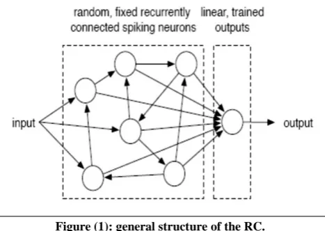
In the recent years the movement prediction had became more demanding in wide fields. Probably the most seemingly fields are the robotic applications such as artificial vision systems and militaries applications specifically in air defense (tracking and predicting movement of rockets and aircrafts). Also a very important application the predictor can be used for; is communication systems' bandwidth reduction in video transmission. Since only the prediction error will be transmitted (like the linear predictor used to reduce the bandwidth in voice transmission in mobile phone) which could be classified as data compression method. The Artificial Intelligent Techniques have reached advanced level that’s enable us to build such systems that require a very strong dynamic behavior and large memory capacity. Experts would prefer to choose AI based technique over a specific design (the later will consume much more time, calculation and effort to be achieved). The Reservoir Computing is a developed technique by [1],[2] under the names of Echo State Network (ESN) and Liquid State Machine (LSM). This neural networks based technique was proven to perform better than any other Dynamic Neural Networks family. But the major difference between the RC tech. and other neural networks is its simple structure and training. The structure consists of two parts; a recurrent neural network with random connection topology usually called the "reservoir". The other part is a feed forward neural network called the "readout layer"; see Figure (1). Its operation based on the following statement: the reservoir computes and process information about the input from

present time to time r (i.e. the last r inputs vectors). Then the readout extracts the information from the reservoir's transition states (there is no stable state in the reservoir [3]). In other words the reservoir transforms temporal information of the input (dynamic characteristics) to spatial information and then the readout classifies or nonlinearly transforms this spatial information to the desired output. The reservoir is scaled rather than trained and only the readout layer is trained using error gradient decent based algorithms or using linear regression method to estimate the readout's weights. The difference between LSM and ESN is the LSM's reservoir's neurons are of the third generation (Spiking neurons); see [4]; while ESN's reservoir's neurons are of the first and/or second generation. The third generation is more biologically inspired than the first and second generation. It was shown in [5] that third generation is more computationally powerful than the second and first generation. Here Movement Predictor was chosen to be implanted using LSM.

3.

MOVEMENT PREDICTION

One would ask how the predictor can predict a movement of an object. The answer is very simple for an advanced biological intelligence (like human beings or some species of animals that developed this ability to hunt other animals) is that they don't take one image but a sequence of images of that object and the background, then forming a time series of images. Every successor image expresses the displacement of the object that it displaced after the predecessor image with respect to time and background which is the first information the brain had got. From the displacement information the brain could obtain the second information by differentiate the displacement with respect to time and background which will result in the speed, similarly the differential of speed with respect to time and background will result in acceleration.

Figure (1): general structure of the RC.

After all these information provided to the brain; it is possible now to predict the movement of an object with some error that varies from almost zero to large values depending on the kind

Note:

 It had been assumed that at the moment of starting of predicting no sudden force should be applied on the moving object or it will be very difficult if not impossible to predict the movement (i.e. if the object suddenly impact an obstacle it will be very hard to predict in which direction and at what speed it will return).

 It should be taken into account the physical properties of the background that may exhibit external forces on the object which in turn decelerates it. This is hard to be mathematically predictable and the brain performs better since the brain concentrates on the behavior of movement which was resulted from that environment to predict the next position rather than mathematical computations.

From the previous note it seems that The Artificial Intelligence is the best alternative for mathematically based systems to replace the brain for this task. Here the LSM as a new AI technique was chosen to be trained as a movement predictor.

4.

TASK SPECIFICATION

It is desired to predict the movement of a uniform black ball on a uniformly polished rectangular white board a few time steps ahead. The ball is with diameter of 16 mm and a mass of 30 grams and the white board area is 22×25.5cm2. The ball was thrown many times with different speeds by a force of human hand from the sides of the board. The probability of the ball being thrown from any side is 1/4 with uniformly distributed probability density functionof ball being thrown from a certain point on a certain side. The ball should not stop on the board (i.e. pass from one side to another for every throw).

5.

SENSORS AND SHOOTING ROOM

The data was supposed to be collected from a 12×16 array of sensors each sensor was with a rectangular shaped aperture. This array was projected to the LSM as an input data in a topographical map. Unfortunately such sensors were not available in local markets. A good alternative was devised for this task called the "Shooting room".

1.1

Shooting room

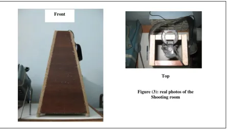
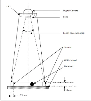
The Shooting room is pyramidical room with rectangular base instead of square base. The top of that pyramid was removed and a digital camera was placed at the upper opening instead. Also the base was removed (i.e. the room has two opens). The slope of walls and the high of the pyramid were set according to some specifications so that the coverage area of the digital camera's lens can cover only the white board area without including any part of pyramid’s walls area. The room's dimensions and real photos are shown in Figure (2) and Figure (3) respectively. The position of digital camera and the coverage angle of its lens with respect to the angles of the pyramid walls are shown in Figure (4); also in this Figure the reader my notice a stands each with high 17mm and base of 15×15mm2 placed at each of Shooting room's corners as a result a gap was formed of 17mm between the white board and the base of the Shooting room. This gap will enable the ball of 16mm diameter to move in a free manner so the digital camera can collect data about its movement. The room was lighted by white LEDs placed at the top of the room (near the camera). Note in Figure (4) the coverage angle of the camera

will cover the whole room's base without including the walls this will ensure that any unnecessary part of image is not included in the data recording process as mentioned earlier. This room was built from wood with a thickness of 13mm and the inner wall was painted in lights brown. The room was stabilized firmly on the white board which was balanced in such a way that the movement of the ball is unbiased toward any direction if no force is used to throw it during data recording process.

The Shooting room and some manipulation in data (which will be discussed in the next Section) will be equivalent to sensors. Another feature of this room is that its isolates the ball from surrounding circumstances that lie outside the room (which in many cases are uncontrollable and changing in short periods such as external light sources, shadows and etc), this will guarantee every image is taken in the same conditions as other images.

1.2

Data recording

The ball was thrown for eighteen times and the camera was filming continuously without stopping between throws. The digital camera was interfaced with the PC using MATLAB Simulink by which some manipulation on the data was achieved as going to be seen later in this section. The resulted data sent to MATLAB Workspace for further processing. This data shall be used as teacher data for the LSM. The interfacing was achieved using a block called "from video device" in Image Acquisition Toolbox. This block was set to capture

RGB1 images with 240 pixels by 320 pixels, 60 image per second and the camera was left to run for 10 seconds (i.e. the size was 240×320×3×(60×10). The first manipulation of data is to convert the RGB video to Intensity video which will result in reduction in size from (240×320×3×600) to (240×320×600). This was done by using a block called "Color Space Conversion" in Video and Image Processing Blockset. The resulted video is further processed by taking the complement of the data using a block called "Image Complement". This block was also found in Video and Image Processing Blockset, for Intensity image this block subtracts each pixel value from the maximum value that can be represented by the input data type and output the difference. After this block, dark areas become light and light areas become dark. For the first sight this step seems to be of no use, but in fact this will make the black ball appears like white and the white board appears in black and since in Intensity image matrix the white color stands for the highest image pixel value and the black color for the lowest image pixel value. This will result in non-zero matrix for the ball movement and almost zero matrix if there no ball presented on the board, finally the data is sent to Workspace for further processing. When using topographic mapping for an image of size (320×240) this will result in a vector of length equal to 76800 which is extremely large, and the reservoir size (as mentioned in [6]) need to be greater than the input vector many times which will be impractical to simulate due to the huge amount of computation required at each time step. Also the ball area is very small compared to the white board area; so many part of the input vector is of no use (i.e. redundant). To solve this problem a very useful function in MATLAB was

1

found called "imresize" this function can reduce the size of image which in this task was set to be from (240×320) to (12×16) (i.e. the same size of sensors array mentioned in the previous Section). The vector length resulted from the topographic mapping is 192 which a reservoir size of 1000 unit could fit into this task. The next step is the subtraction of a freeze image (image of no ball over the white board) from every image constituting the video, this step will remove unwanted object other than the ball such as stains, pitches and scratches on the board. The resulted movie was played and any image without the ball was discarded manually and bookmarks were added to separate each example2 from the next one. Five freeze images were added after each example to force the reservoir to settle and so making it ready to receive the next example. This has resulted in a movie of length equal to 319 (i.e. 319 images) and each image was topographically mapped to form the teacher output data with a size of (192×319). The teacher input data is then formed by placing a number of freezes images equal to the number of images wanted to predict ahead (each image means a time of (1/60) second) before the teacher output which will result in a size of (192×(319+number of freezes images added before the teacher output)). Now these data are ready to be used to train the LSM as a movement predictor.

Note:

 in this simulation it was chosen to predict one image ahead or (1/60) sec., this time can be increased as much as needed taking into account this will increase the prediction error, to reduce the prediction error as much as possible all what have to be done is increasing the dynamics of the reservoir.

6.

RESERVOIR SPECIFICATIONS AND

PARAMETERS

The LSM reservoir units are Spiking neurons instead of Analog neurons, so for input vector of length equal to 192 a reservoir size of 1000 spiking neurons is a good choice. Two LSMs are chosen for simulation, the first network is with Connectivity of 5% (connection fraction of 0.05) and λmax

(Spectral radius) equal to 0.1, the second network is with Connectivity of 40% (connection fraction of 0.4) and λmax

equal to 0.9; it will be referred to these LSMs by LSM #1 and LSM #2 respectively. 20% of the spiking neurons where chosen to be inhibitory (the other 80% are excitatory) and the reservoir excitatory weight matrix's (Wexitatory) non-zero elements were chosen from {0.3, 0.8, 0.5} with equally likely probability equal to (connection fraction×1000 /3000) for excitatory and for inhibitory weight matrix's (Winhibitory) non-zero elements were chosen from {-0.4, -0.7, -0.9} with equally likely probability equal to (connection fraction×1000 /3000). The total reservoir weight matrix (W) is created by concatenate (Wexitatory) and (Winhibitory) in row wise manner. For this simulation the "leaky Integrate-and-fire"; see [4]; spiking neuron model was chosen with the following specifications:

1) Threshold voltage (ϑ) is set to 15 mV. 2) Reset voltage ( )is set to-6 mV.

2

Example means the action from the moment of ball's entrance to the moment of ball's departure. The number of examples equal to the number of throws.

3) Refractory period: the absolute refractory period (δ ) is set to be 3 msec. (or three time steps by assuming one time step in the program equal to 1msec), the negative refractory period () time constant equal to and taking only the effect of the last spike occurring (i.e. the spiking neuron has a short term memory).

4) Membrane impulse response was chosen to be . 5) The synapse impulse response was chosen to

be .

6) R=166MΩ and C=60 pF.

.

Note:

 All reservoir neurons are assumed to have the same parameters.

If the weight connecting two neurons (from predecessor neuron to successor neuron) is negative then the predecessor neuron is classified as inhibitory neuron otherwise it is classified as excitatory neuron (i.e. the sign of the weight defines the class and every neuron has the same parameters). This is not true in biological nervous systems because every neuron might have different parameters and many synaptic connections with other single neuron are allowed, these synaptic connections are with different weights (which they are always positive), time delays and synaptic impulse responses. These aspects could be taken into account in other simulations but not in this one due to huge amount of computation required to implement it.

The input weight matrix's (Win) elements are randomly set between 20 and 0 with uniform distribution probability

density function3, the analog input was injected using the

external input method [6], this step is very useful since the coding stage is not needed any more.

The readout layer constituted of 192 sigmoidal neurons (the same size of the output vector); the spiking activity of the reservoir (or reservoir states (x)) is not directly treated since the readout analog neurons cannot cope with spikes as an input to them, so the reservoir states is transformed to analog domain. This was done by filtering each state with the filter of impulse response where τr is set to 10 msec. It will

denoted to the response of this filter to the reservoir's state by "intermediate", then AWGN was inserted with zero mean and 10-5 variance to the output of this filter. Note that other impulse responses for this filter can be used for this task and various impulse responses are also allowed to be used in the same reservoir. After this step the readout is ready to be trained, the linear regression training method was selected for this task.

3

Figure (2): the dimensions of Shooting room

Top

Figure (4): the set up of the Shooting room with all equipment to record data.

7.

BASED AND EVENT BASED

SIMULATIONS

Time based and Event based simulations could both be implemented to simulate the LSM even though the Event based is the most appropriate since the temporal information in spike pattern is still preserved due to that the Event based simulation schedule the time's instants that supposed to have a

new event4 and then performs the computations only at the

scheduled time's instants. This means any time step without event does not require the program to stop at them and perform operation; this seems to be reasonable since it does not operate the processor at unnecessary time's instants which will result in shorter running period with minimum lost of information. Unfortunately this kind of simulation could not be done using MATLAB without any interfacing with other programming languages (usually the C or C++_{). This obstacle} was avoided by some modifications on the arrangement of the LSM's simulation program. These modifications are:

1) Regard every ten time steps in MATLAB is one time step for every input vector (i.e. use the same input vector for ten consecutive time steps in MATLAB).

2) Sample the filtered reservoir's states every ten time steps and train the readout to map the desired output from

4 _{In this context event means something new had}

happened to the variables of the systems.

these samples and not from the whole history of the filtered reservoir' states.

After these modifications the spike from state (xi) is free to

appear at any time step for one or many time within every consecutive ten time steps, even though it is still time based simulation and if further accuracy is needed all what have to be done is to replace the ten time steps with higher values, but this increase will slow down the execution of the program since the total time steps in the program will increase, so a compromise have to be done between accuracy and time. The choice for this simulation was ten time steps.

Note:

 for Event based simulation the states of the reservoir are written in the form of x(t) and for time based in the form of x(n) since the Event based simulation uses the exact timing and the time based simulation uses the fixed time steps to perform computations.

8.

SIMULATION RESULTS

As mentioned earlier in Section (5) the length of the output vector of the LSM is 192 this vector was inversely topographically mapped into 12×16 matrix, the resulted movie size was (12×16×319). When this movie was played, it was difficult to watch the predicted ball's movement due to its low quality and thus comparing it with the original movie which was of size (240×320×319) (before manipulations discussed in Section (5)), so in order to compare; the resulted movie was resized to be (240 ×320×319).

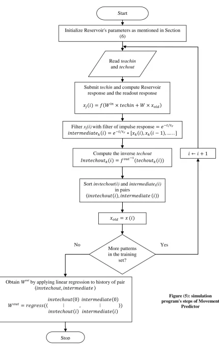
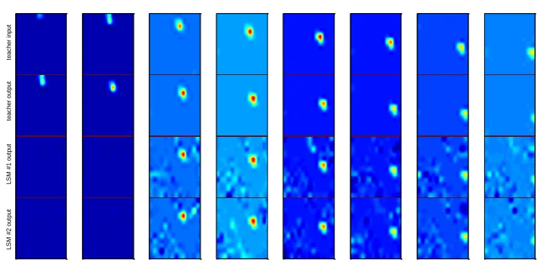
second one is by viewing images from the moment of throwing the ball to the moment of disappearing it with excluding every freeze images, the third one is by writing the Mean Square Error (MSE) of every example and then averaging the MSE of each example alone. Only the Testing result will be viewed, the first fifteen images may be regarded as a transient period and so will be discarded. Viewing images will be in four windows concatenated in vertical way and separate from each other by a horizontal line, the upper window shows ball position (teacher input), the second window shows an advanced ball position (teacher output) and the last two windows shows the predicted position by LSM #1 and LSM #2 respectively. A very important option must be mentioned which is the color mapping option. This option may increase the ability of the reader to notify the differences in images. It has been found that the "jet" color map was a very appropriate for this task; even thought if the reader had downloaded the movie from the author then it is easy to change it to other color maps. The flowchart shown in Figure (5) shows the simulation program's steps, where techin and techout denotes the teacher input and teacher output respectively, xold and x denotes the old and present reservoir

states respectively, xj is j-th component of present state (x), f

and are the activation functions of reservoir and readout layer respectively (both are sigmoidal), invtechout is the inverse of techout by the function (the inverse function of ), intermediatek denotes the k-th component of

intermediate and "*" denotes the convolution operation. As mentioned in Section (5) the movie was split into examples, each example starts at the moment of the existence of the ball on the white board and ends after the insertion of five freezes images when the ball departs. Only specific parts of example will be viewed, these parts are from the moment of the existence of the ball at one of the edges for the teacher input to the moment of departure of the ball from one of the edges for the teacher output.

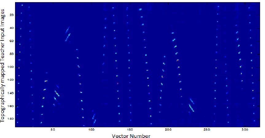
The simulation results of LSM #1 and LSM #2 trained to predict (1/60) second ahead for fourteen examples are shown in Table (1). For shortness, it was chosen to view the resulted images for only four examples; see Figure (6). The resulted images for all examples are shown in [6]. From Table (1) it can be seen that there is no much difference between the two machines' results even with the relatively large difference in their Connectivities and Spectral radiuses. This could be explained by the low prediction time required from both machines and due to the effect of five freezes images added between examples. The reader can notice the differences in the reservoirs' firing activities with respect to teacher input vectors' history in Figure (7); taking into account every one time step in the teacher input history equal to ten time steps in the reservoirs. In Figure (7) it can be noticed LSM #2 has higher firing activity for more extended period of time (wider stripes) than LSM #1 since machine #2 has higher λmaxthan

machine #1 and so a richer dynamics and memory capacity. For further exploration of LSM's features another simulation will be carried out, but now for a prediction time of (4/60) second ahead (or four images ahead). Three reservoirs will be used this time; the first will be one of the machines used in the previous simulation (LSM #2); the second machine will be with a size of 1000 units, Connectivity of %10 and with λmax

equal to 1.3 and will be donated by LSM #3. The third machine with a size of 2000 units, Connectivity of %40 and with λmax equal to 0.9 and will denote by LSM #4.

Note:

 LSM #1 was excluded from this competition due to its low spectral radius and so it low memory

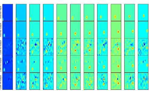
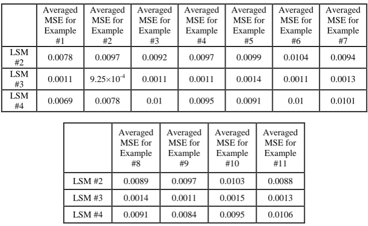
capacity since this task requires a higher memory capacity due to the relatively high prediction time. Unlike the previous simulation the averaged MSE will be calculated from the moment at which all the machines start to predict. All short examples (examples with period less than or equal to four images) will be excluded because in these examples the ball in the teacher output will disappear before it appears in the teacher input. Only eleven examples had remained from fourteen. Again, for shortness only four examples were chosen to be viewed. The simulation results are shown in Figure (8) and Table (2); the reader can see the other example by mailing to author asking to download the images. From Figure (8) and Table (2) it can be noticed that LSM #3 has better performance than LSM #2 and LSM #4, the last two have a quite similar performances even with the large difference in their sizes. The reservoirs' firing activities and the teacher input history of the three machines are shown Figure (9). It can be seen that both LSM #2 and LSM #4 almost have the same firing activities, and theirs firing activities are extended for the same period of time even with the large difference in their sizes. LSM #3 has the highest firing activity with more extended period of time than the previous machines. This extension in time causes the firing activity resulted from one example to interfere with the firing activity resulted from the next example, and since the static readout layer had been trained to extract the desired output from a certain pattern (which in this case can be changed if the sequence of examples is manipulated) which will lead in the failure of the machine to produce the desired output (i.e. the machine is trained to produce the desired output according to a certain sequence of examples and not at a certain single example). This issue can be regarded as a major weakness point for LSM #3. This weakness point can be avoided if the number of freezes images between examples is increased (i.e. increasing the resting period of the machine). This would make the system impractical for real-time applications.

After this statement one can regard LSM #2 as the winner in this competition over LSM #3 and

LSM #4 (the later suffers from the high complexity due to its large size). Table (3) shows the machines main parameters, names and simulation time.

9.

DISCUSSION

From Figures (6), (8) and Tables (1), (2) it can be conclude that the LSM has succeeded as a Movement Predictor for both short and long term prediction using analog input without coding . Also it is possible to use time based simulation without the need to interface with other programming languages.

It was shown that how the Spectral radius (λmax) value could

Start

Initialize Reservoir's parameters as mentioned in Section (6)

Submit techin and compute Reservoir response and the readout response

Compute the inverse techout

Sort invtechout(i) and intermediatek(i)

in pairs Read teachin

and techout

Yes

No

More patterns in the training

set?

Obtain Wout by applying linear regression to history of pair

Stop No

Filter xj(i)with filter of impulse response

Figure (5): simulation program's steps of Movement

Table (1): Recorded result for LSM #1 and LSM #2. Averaged MSE for Example #1 Averaged MSE for Example #2 Averaged MSE for Example #3 Averaged MSE for Example #4 Averaged MSE for Example #5 Averaged MSE for Example #6 Averaged MSE for Example #7

LSM #1 0.0018 0.0015 0.0018 0.0019 0.0015 0.0015 0.0013

LSM #2 0.0019 0.0013 0.0019 0.002 0.0015 0.0019 0.0014

Averaged MSE for Example #8 Averaged MSE for Example #9 Averaged MSE for Example #10 Averaged MSE for Example #11 Averaged MSE for Example #12 Averaged MSE for Example #13 Averaged MSE for Example #14

LSM #1 0.0018 0.0017 0.0019 0.0018 0.0018 0.0018 0.0014

LSM #2 0.0019 0.0019 0.0018 0.002 0.0021 0.0019 0.0014

Figure (6.a): Example #1

Figure (6.b): Example #2

Figure (6.c): Example #3

Figure (6.d): Example #4

Figure (6): simulation results of four examples for LSM #1 and LSM #2.

L

S

M

#

2

o

u

tp

u

t

L

S

M

#

1

o

u

tp

u

t

t

e

a

c

h

e

r

o

u

tp

u

t

te

a

c

h

e

r

in

p

u

t

L

S

M

#

2

o

u

tp

u

t

L

S

M

#

1

o

u

tp

u

t

t

e

a

c

h

e

r

o

u

tp

u

t

te

a

c

h

e

r

in

p

u

Figure (7.a): firing activity of LSM #1

Figure (7.c): teacher Input vectors' history

Figure (7): the firing activities for a) LSM #1 b) LSM #2 respectively. c) The teacher input vectors' history.

Figure (8.a): Example #1

L

S

M

#

4

o

u

t

p

u

t

L

S

M

#

3

o

u

t

p

u

t

L

S

M

#

2

o

u

t

p

u

t

t

e

a

c

h

e

r

o

u

t

p

u

t

t

e

a

c

h

e

r

in

p

u

Figure (8.b): Example #2

Figure (8.c): Example #3

L

S

M

#

4

o

u

t

p

u

t

L

S

M

#

3

o

u

t

p

u

t

L

S

M

#

2

o

u

t

p

u

t

t

e

a

c

h

e

r

o

u

t

p

u

t

t

e

a

c

h

e

r

in

p

u

t

L

S

M

#

4

o

u

tp

u

t

L

S

M

#

3

o

u

tp

u

t

L

S

M

#

2

o

u

tp

u

t

te

a

c

h

e

r

o

u

tp

u

t

te

a

c

h

e

r

in

p

u

Figure (8.d): Example #4

Figure (8): simulation results of four examples for LSM #2, LSM #3 and LSM #4.

Table (2): Recorded results for LSM #2, LSM #3 and LSM #4.

Averaged MSE for Example

#1

Averaged MSE for Example

#2

Averaged MSE for Example

#3

Averaged MSE for Example

#4

Averaged MSE for Example

#5

Averaged MSE for Example

#6

Averaged MSE for Example

#7 LSM

#2 0.0078 0.0097 0.0092 0.0097 0.0099 0.0104 0.0094

LSM

#3 0.0011 9.25×10 -4

0.0011 0.0011 0.0014 0.0011 0.0013

LSM

#4 0.0069 0.0078 0.01 0.0095 0.0091 0.01 0.0101

Averaged MSE for Example

#8

Averaged MSE for Example

#9

Averaged MSE for Example

#10

Averaged MSE for Example

#11

LSM #2 0.0089 0.0097 0.0103 0.0088

LSM #3 0.0014 0.0011 0.0015 0.0013

LSM #4 0.0091 0.0084 0.0095 0.0106

L

S

M

#

4

o

u

tp

u

t

L

S

M

#

3

o

u

tp

u

t

L

S

M

#

2

o

u

tp

u

t

te

a

c

h

e

r

o

u

tp

u

t

te

a

c

h

e

r

in

p

u

Table (3): Machines main parameters, names and simulation time.

LSM #1 LSM #2 LSM #3 LSM #4

Spectral radius (λmax) 0.1 0.9 1.3 0.9

Connectivity 5% 40% 10% 40%

Reservoir' size 1000 1000 1000 2000

Simulation time required for first task 162 minute

168

minute - -

Simulation time required for second

task -

158

minute 163 minute 341 minute

Figure (9.a): firing activity of LSM #2

Figure (9.c): firing activity of LSM #4

Figure (9.d): teacher input vector's history

10.

REFERENCES

[1] H. Jaeger, “The echo state approach to analyzing and training recurrent neural networks,” Technical Report GMD Report 148, German National Research Center for Information Technology, 2001.

[2] W. Maass, T. Natschlaeger and H. Markram., “Real-time computing without stable states: A new framework for neural computation based on perturbations,” Neural Computation, 14(11), pp. 2531-2560, 2002.

[3] T. Natschlager, W. Maass and H. Markram, “The 'Liquid computer': A Novel Strategy for Real-Time Computing on Time Series,” Journal Article, Special Issue on Foundations of Information Processing of {TELEMATIK}, 2002.

[4] W. Maass and C. M. Bishop, Pulsed Neural Networks, MIT-press, 1999.

[5] W. Maass, “Noisy spiking neurons with temporal coding have more computational power than sigmoidal neurons,” Advances in Neural Information Processing Systems, vol. 9, p. 211–217, 1997.

[6] A. S. Abdulrasool, A Study of Reservoir Computing: Echo State Network and Liquid State Machine, Bghdad University, Electrical Engineering Department, M.Sc. thesis, 2010.

[7] W. Maass, T. Natschlaeger, and H. Markram., “Real-time computing without stable states: A new framework for neural computation based on perturbations,” Neural Computation, 14(11), pp. 2531-2560, 2002.

[8] A.V. Holden, J.V. Tucker and B.C. Thompson, “Can excitable media be considered as computational systems?.,” Physica D, 1991.

[9] T. Natschlager, W. Maass and H. Markram, “The 'Liquid computer': A Novel Strategy for Real-Time Computing on Time Series,” Journal Article, Special Issue on Foundations of Information Processing of {TELEMATIK}, 2002.

[10] J. M. Zurada, Introduction to Artificial Neural Systems, West Publishing Company, 1992.

[11] B. Schrauwen, Towards Applicable Spiking Neural Networks, Doctrine assertion, Gent University of Technology, 2008.

[12] W. Maass, “Noisy spiking neurons with temporal coding have more computational power than sigmoidal neurons,” Advances in Neural Information Processing Systems, vol. 9, p. 211–217, 1997.

[13] W. Maass, “Networks of spiking neurons: the Third Generation of Neural Network Models,” Neural Networks, vol. 10, no. 9, p. 1659–1671, December 1997. [14] W. Maass, T. Natschlger and H. Markram, “Fading

memory and kernel properties of generic cortical microcircuit models,” Journal of Physiology, 98(4-6), pp. 315-330, 2004.

[15] W. Maass, “Lower bounds for the computational power of networks of spiking neuron,” Neural Computation, 8(1), pp. 1-40, 1996.

[16] J. Triesch, “Synergies between intrinsic and synaptic plasticity mech-anisms,” Neural Computation, 19, p. 885–909, 2007.

[17] W. Maass and C. M. Bishop, Pulsed Neural Networks, MIT-press, 1999.

[18] E. O.Dijk, Analysis of Recurrent Neural Networks with Application to Speaker Independent Phoneme Recognition, University of Twente, M.Sc thesis, 1999 .

[19] R. B. Randall and Jens Hee, “Cepstrum Analysis,” Technical Review No. 3, 1981.

[20] A. Gupta, Y. Wang and H. Markram, “Organizing principles for a diversity of GABAergic interneurons and synapses in the neocortex,” Science (New York, N.Y.), Vol. 287, No. 5451, pp. 273-278, 14 January 2000. [21] Chatterjee, S. and A.S. Hadi, “Influential

Observations,High Leverage Points, and Outliers in Linear Regression,” Statistical Science 1(3), pp. 379-416, 1986.

[22] A. Turing, Intelligent Machinery, C. E. a. A. Robertson, Ed., Reprinted in "Cybernetics: Key Papers.", 1948, p. 31.

[23] Draper N. and H. Smith, Applied Regression Analysis, 2nd ed., Wiley, 1981.

[24] Lukoševičius, M., and H. Jaeger, “Reservoir computing approaches to recurrent neural network training,” Science Review 3 (3), pp. 127-149, 2009.

[25] Bernhard Scholkopf and Alex J. Smola, Learning with Kernels: Support Vector Machines, Regularization, Optimization and Beyond, MIT press, 2002.

[26] Jaeger, H., “Short term memory in echo state networks,” Tech. rep. no.GMD report 152.German National Research Center for Information Technology, 2001.

[27] Jaeger, H., “The echo state approach to analyzing and training recurrent neural networks,” Technical Report GMD Report 148, German National Research Center for Information Technology, 2001.

[28] J. J. Steil, “Backpropagation-Decorrelation: online recurrent learning with O(N) complexity,” in Neural Networks, Proceedings, IEEE International Joint Conference on, 2004.

[29] A. B. Atiya and A. G. Parlos, “New results on recurrent network training:Unifying the algorithms and accelerating convergence,” IEEE Trans.Neural Networks, vol. 11, no. 9, pp. 697–-709, 2000.

[30] D. Verstraeten, B. Schrauwen, M. D'Haene and D. Stroobandt, “An experimental unification of reservoir computing methods,” Neural Networks, 29, pp. 391-403, 2007.

[31] S. Thorpe, A. Delorme, V. Rullen and R., “Spike based strategies for rapid processing,” Neural Networks, vol. 14(6-7),, pp. 715-726, 2001.